To analyze the effects of pollution, Mexico City was divided into
five zones. The function get_zone_imeca can download data
for each zone measured in IMECAs, as opposed to the original units used
by get_station_data.
## Auto-install required R packages
if (!require("pacman")) install.packages("pacman")
## Loading required package: pacman
pacman::p_load(aire.zmvm, dplyr, ggplot2)
## The mxmaps package must be installed from GitHub:
## if (!require("devtools")) {
##     install.packages("devtools")
## }
## devtools::install_github("diegovalle/mxmaps")
library(mxmaps)

df <- zones
df$value <- df$zone

p <- mxmunicipio_choropleth(df, num_colors = 6,
                       zoom = df$region,
                       title = "Geographic Zones of Mexico City") +
  scale_fill_manual("Zone", values = c("Centro" = "#e41a1c", "Noreste" = "#377eb8",
                               "Noroeste" = "#4daf4a",
                               "Sureste" = "#984ea3",
                               "Suroeste" = "#ff7f00"))
## Scale for fill is already present.
## Adding another scale for fill, which will replace the existing scale.
plot(p)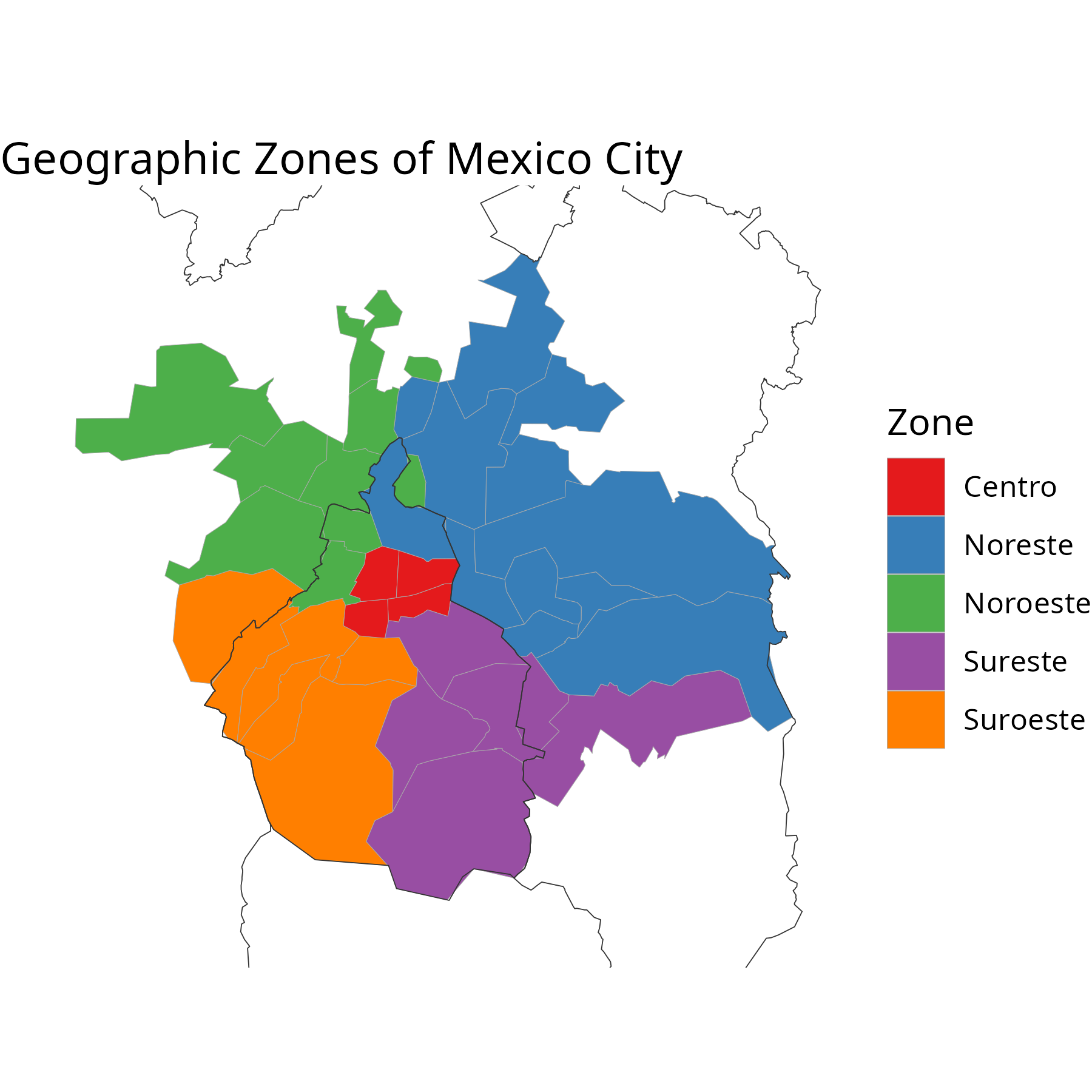
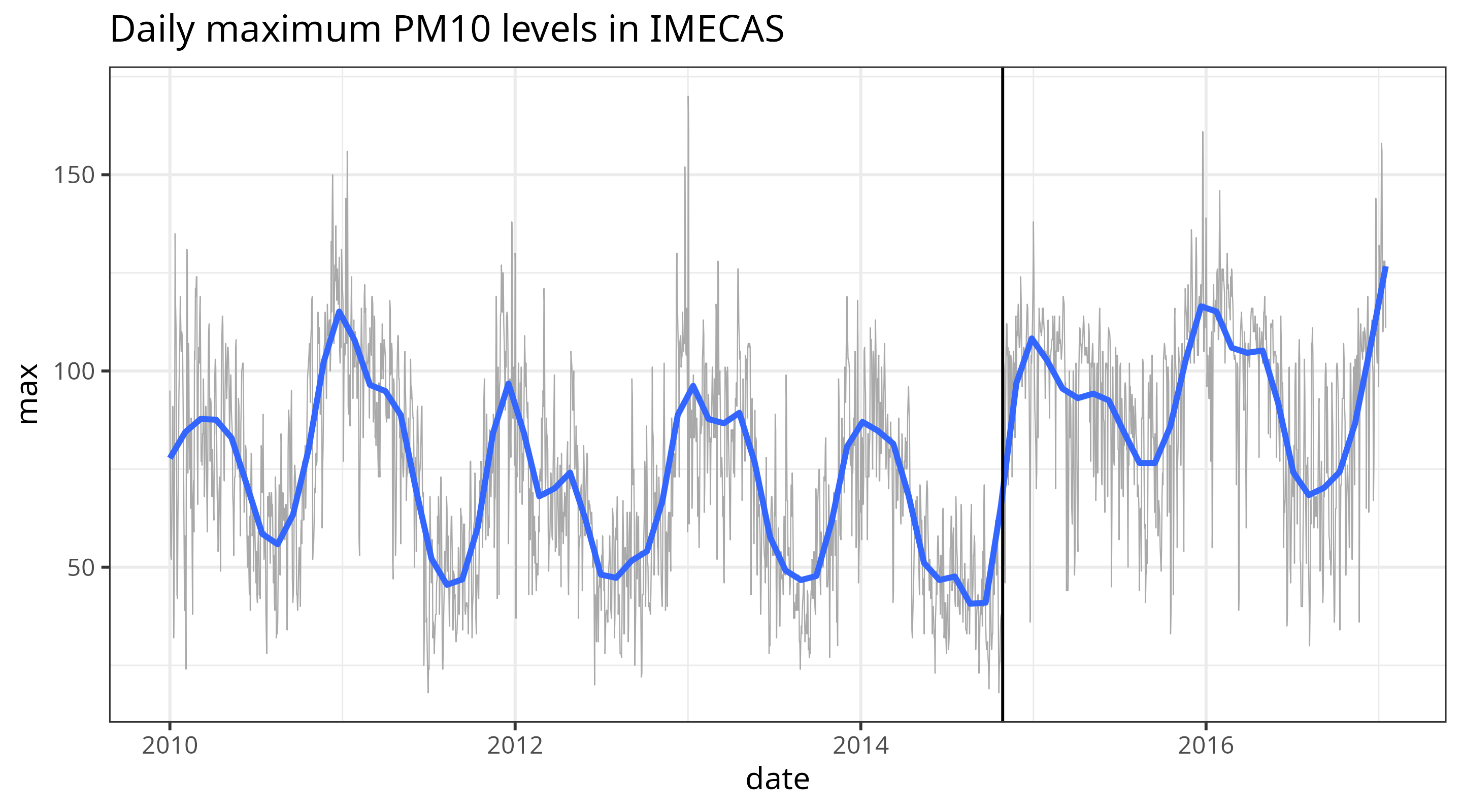
Note that the standards for measuring PM10 and O3 in IMECAs changed in October 2014, and the function prints a message.
# Download pm10 data since 2008 for all available zones ("TZ")
pm_10 <- get_zone_imeca(criterion = "MAXIMOS", # Can be MAXIMOS (daily maximum) or
                                              # HORARIOS (hourly average)
                       pollutant = "PM10", # "SO2", "CO", "NO2", "O3", "PM10",
                                           # "TC" (All pollutants)
                       zone = "TZ", # "NO", "NE", "CE", "SO", "SE", "TZ" (All zones)
                       start_date = "2010-01-01", # Can't be earlier than 2008-01-01
                       end_date = "2017-01-15") # Can be up to the current date
## Starting October 28, 2014 the IMECA values for O3 and PM10 are computed using NOM-020-SSA1-2014 and NOM-025-SSA1-2014| date | zone | pollutant | unit | value |
|---|---|---|---|---|
| 2010-01-01 | NO | PM10 | IMECA | 89 |
| 2010-01-02 | NO | PM10 | IMECA | 57 |
| 2010-01-03 | NO | PM10 | IMECA | 44 |
| 2010-01-04 | NO | PM10 | IMECA | 23 |
| 2010-01-05 | NO | PM10 | IMECA | 38 |
| 2010-01-06 | NO | PM10 | IMECA | 56 |
Plotting the data makes the change that took place in October 2014 very obvious:
# Plot the overall highest maximum pm10 level with trendline
ggplot(pm_10 %>% group_by(date) %>% summarise(max = max(value, na.rm = TRUE)),
                      aes(date, max, group = 1)) +
  geom_line(color = "darkgray", linewidth = .2) +
  geom_smooth(method = "gam", formula = y ~ s(x, k = 50), se = FALSE) +
  ggtitle("Daily maximum PM10 levels in IMECAS") +
  geom_vline(xintercept = as.Date("2014-10-28")) +
  theme_bw()