Introduction to the aire.zmvm package

This document introduces you to tools for downloading data from each of the pollution, wind and temperature measuring stations in the Zona Metropolitana del Valle de México (greater Mexico City).

Core Functions

The basic set of functions provided by the package:

get_station_data and get_station_month_data download pollution, wind and temperature data for each of the measuring stations in the original units (ppb, µg/m³, etc).
get_station_imeca download pollution values for each station in IMECAs
get_zone_imeca download pollution data in IMECAs for each of the 5 geographic zones of Mexico City
get_latest_imeca download the latest pollution hourly maximums for each of the measuring stations.
idw360 inverse distance weighting modified to work with degrees, useful for wind data

Because of limitations with the SEDEMA website http://www.aire.cdmx.gob.mx/ (where all data downloaded by the aire.zmvm comes from), options for each of the function aren’t entirely consistent but hopefully the following table will make them clearer.

function	date range	Units	Wind / Tmp / RH	Earliest Date	Pollutants	Includes All Stations	Criterion
get_station_data	years	Original	Yes	1986	SO2, CO, NO2, O3, PM10, PM25, WSP, WDR, TMP, RH	Yes	hourly, daily maximum, daily minimum
get_station_month_data	1 month	Original	Yes	2005‑01	SO2, CO, NO2, O3, PM10, PM25, WSP, WDR, TMP, RH	Yes	hourly, daily maximum, daily minimum
get_station_imeca	1 day	IMECA	No	2009‑01‑01	SO2, CO, NO2, O3, PM10	No	hourly
get_zone_imeca	1 or more days	IMECA	No	2008‑01‑01	SO2, CO, NO2, O3, PM10	Only zones	hourly, daily maximum
get_latest_imeca	1 hour	IMECA	No	Latest only	Maximum value of SO2, CO, NO2, O3, PM10	No	latest hourly

Map of Pollution Levels

Pollution is monitored by a series of stations located throughout the Mexico City Metro Area. Since there are different pollutants to monitor, each measured in different units, and each with different specified averaging periods, a common scale called IMECA was created to make them comparable. If pollutants reach 151 IMECA points or more the Mexico City government can declare a phase I smog alert and order cars off the streets and place limits on polluting industries.

On May 4, 2018 there was a smog alert, but there wasn no doble hoy no circula because metereological conditions were forecast to improve the next day. We’ll show just how easy it is to make a map of pollution levels during the alert with this package.

First we load the packages we need to run this vignette and download the pollution data:

library("aire.zmvm")
library("lubridate")
library("dplyr")
library("ggplot2")
library("ggmap")
library("sp")
library("gstat")

# Download hourly data for all pollutants during May 04, 2018 
# The maximum Ozone level was reached at 17:00 PM local time,
# 16:00 with no daylight savings time
ldf <- lapply(c("PM10", "O3", "SO2", "NO2", "CO"),
              function(x) get_station_imeca(x, "2018-05-04") %>%
                filter(hour == 16) )

Here’s what the data we just downloaded looks like:

date	hour	station_code	pollutant	unit	value
2018-05-04	16	HGM	O3	IMECA	175
2018-05-04	16	IZT	O3	IMECA	165
2018-05-04	16	MER	O3	IMECA	154
2018-05-04	16	BJU	O3	IMECA	152
2018-05-04	16	UAX	O3	IMECA	144
2018-05-04	16	UIZ	O3	IMECA	125
2018-05-04	16	CCA	O3	IMECA	121
2018-05-04	16	PED	O3	IMECA	115
2018-05-04	16	AJM	O3	IMECA	111
2018-05-04	16	NEZ	O3	IMECA	106

You may have noticed that the code comments mention the local time as being 1 hour ahead of that returned by the function. That’s because the hourly data returned by get_station_imeca comes in a format that is not affected by daylight savings time—i.e. 6 hours behind UTC (Etc/GMT+6). If, for example, you ever want to analyze pollution levels at peak commuting times, you’ll want to convert the time to the local timezone of America/Mexico_City. You can use the following code to do the conversion:

format(as.POSIXct("2017-05-04 16:00", tz = "Etc/GMT+6"),
       tz = "America/Mexico_City",
       usetz = TRUE)
#> [1] "2017-05-04 17:00:00 CDT"

The package also includes a data.frame named stations that includes the latitude and longitude of all pollution measuring stations.

station_code	station_name	lon	lat	altitude	comment	station_id
ACO	Acolman	-98.91200	19.63550	2198		484150020109
AJU	Ajusco	-99.16261	19.15429	2942		484090120400
AJM	Ajusco Medio	-99.20774	19.27216	2548		484090120609
ARA	Aragón	-99.07455	19.47022	2200	Finalizó operación en 2010	484090050301
ATI	Atizapan	-99.25413	19.57696	2341		484150130101

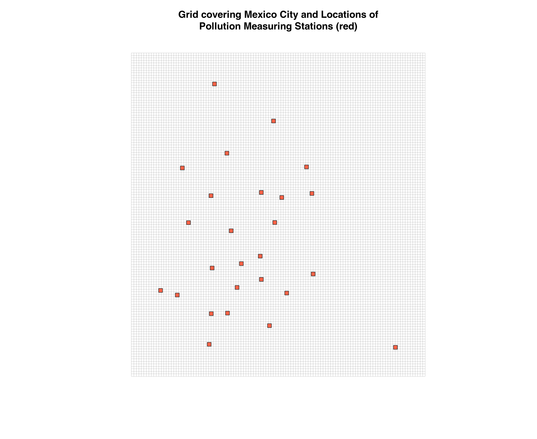
We will use this data to create a grid covering Mexico City and extrapolate the pollution values to each cell in the grid by inverse distance weighting from the locations of the measuring stations.

create_grid <- function(station_vec, pixels = 1000) {
  df <- stations[stations$station_code %in% station_vec,]
  geog <- df[,c("lat", "lon")]
  coordinates(geog) <- ~lon+lat
  proj4string(geog) <- "+proj=longlat +datum=WGS84 +no_defs +ellps=WGS84 +towgs84=0,0,0"
  ## Add a margin surrounding the stations
  geog@bbox <- bbox(geog) + c(-0.05, -0.05, 0.05, 0.05)
  geog.grd <- makegrid(geog, n = pixels)

  grd.pts <- SpatialPixels(SpatialPoints(geog.grd))
  as(grd.pts, "SpatialGrid")
}


# Sometimes stations are taken offline for maintenance, exclude those
# that weren't reporting data
reporting_stations <- unique(na.omit(do.call(rbind, ldf))$station_code)
# 50x50 grid covering Mexico City
grid <- create_grid(reporting_stations, 15000)

plot(grid, main = "Grid covering Mexico City and Locations of\nPollution Measuring Stations (red)",
     col = "#666666", lwd = .2)
# Plot the locations of the stations
geog <- stations[stations$station_code %in% reporting_stations, c("lat", "lon")]
coordinates(geog) <- ~lon+lat
points(geog, pch = 22, col = "#333333", bg = "tomato1", cex = 1.2)

There are probably additive or interaction effects between pollutants, but to keep things simple we’ll do like the Mexico City government when it reports pollution levels and simply ignore them. We’ll take the maximum pollution value in each cell of the grid to create the map.

heatmap <- function(df, grid){
  if(nrow(df) == 0){
    return(data.frame(var1.pred = NA, var1.var = NA, lon = NA, lat = NA))
  }

  df <- left_join(df, stations, by = "station_code")
  df <- df[!is.na(df$value),]
  df <- df[,c("lat", "lon", "value")]
  coordinates(df) <- ~lon+lat
  # For radiation pollution the exponent should be 2
  # See http://www.sciencedirect.com/science/article/pii/S009830041200372X
  df.idw <- idw(value ~ 1, df, grid, idp = 2, debug.level = 0)

  idw = as.data.frame(df.idw)
  names(idw) <- c("var1.pred", "var1.var", "lon", "lat")

  idw
}


# Create the IDW heatmap for each pollutant
idw_tiles <- lapply(ldf, heatmap, grid)
# Calculate the maximum value across all pollutants
maxes <- apply(do.call(cbind, lapply(idw_tiles,
                                     function(x) x[["var1.pred"]])),
               1, max)
idw_tiles_max <- data.frame(var1.pred = maxes,
                       lat = idw_tiles[[1]]$lat,
                       lon = idw_tiles[[1]]$lon)

Plot

Now we will use the package ggmap to plot the locations of the stations and the pollution grid on top of a map. Note that you may have to install a beta version of ggmap by running: devtools::install_github("dkahle/ggmap", ref = "tidyup")

qmplot(x1, x2, data = data.frame(grid), geom = "blank",
       maptype = "toner-lite", source = "stamen", zoom = 10)  +
  geom_tile(data = idw_tiles_max, aes(x = lon, y = lat, fill = var1.pred),
            alpha = .8) +
  scale_fill_gradient2("IMECA",
                       low = "#abd9e9",
                       mid = "#ffffbf",
                       high = "#f46d43",
                       midpoint = 100) +
  geom_point(data = stations[stations$station_code %in% reporting_stations, ],
             aes(lon, lat), shape = 22, size = 1.6) +
  ggtitle(paste0("Pollution in Mexico City during the pollution",
                 " emergency of May 4, 2018"))

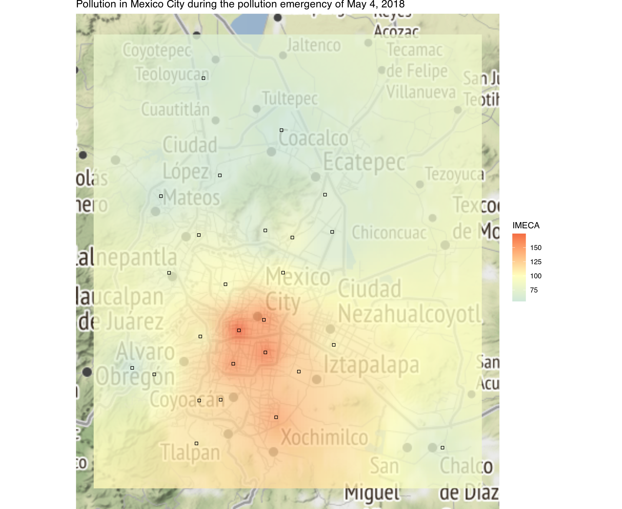
Map of Pollution in Mexico City

Diego Valle-Jones

2020-07-31

Core Functions

Map of Pollution Levels

Plot