Hoy no circula

In an effort to lower pollution levels, the Mexico City government introduced the Hoy No Circula program in 1989, which bans most cars from circulating once a week. But did it really work?

Station data

The function get_station_data can be used to download pollution and wind data going back to 1986. However, not all pollutants are available that far back; requesting a pollutant that is unavailable will result in a warning.

## Auto-install required R packages
if (!require("pacman")) install.packages("pacman")

## Loading required package: pacman

pacman::p_load(aire.zmvm, dplyr, ggplot2, mgcv, lubridate, stringr,
               gridExtra, zoo, sp, mapproj)

download_data <- function(pollutant) {
  #print(paste0("Downloading data for: ", pollutant))
  suppressWarnings({
    o3 <- get_station_data(criterion = "MAXIMOS", # Can be MAXIMOS (daily maximum), 
                           # MINIMOS (daily minimum), 
                           # or HORARIOS (hourly average)
                           pollutant = pollutant, # "SO2", "CO", "NOX", "NO2", "NO", "O3", 
                                                  # "PM10", "PM25", "WSP", "WDR", "TMP", "RH"
                           year = 1986:2018, # The earliest year allowed is 1986
                           progress = FALSE)
  })
  o3$pollutant <- pollutant
  # Daily max among all base stations
  o3 %>% 
    group_by(date, pollutant) %>% 
    summarise(max = ifelse(all(is.na(value)),
                           NA,
                           base::max(value, na.rm = TRUE))) %>%
    na.omit() %>%
    ungroup()
}

ll <- mapply(download_data, 
             pollutant = c("NO", "SO2", "CO", "NOX", "NO2", "O3", "PM10", "PM25"),
             SIMPLIFY = FALSE)
df_maximos <- bind_rows(ll)
knitr::kable(head(df_maximos))

date	pollutant	max
2003-01-01	NO	201
2003-01-02	NO	228
2003-01-03	NO	229
2003-01-04	NO	301
2003-01-05	NO	230
2003-01-06	NO	275

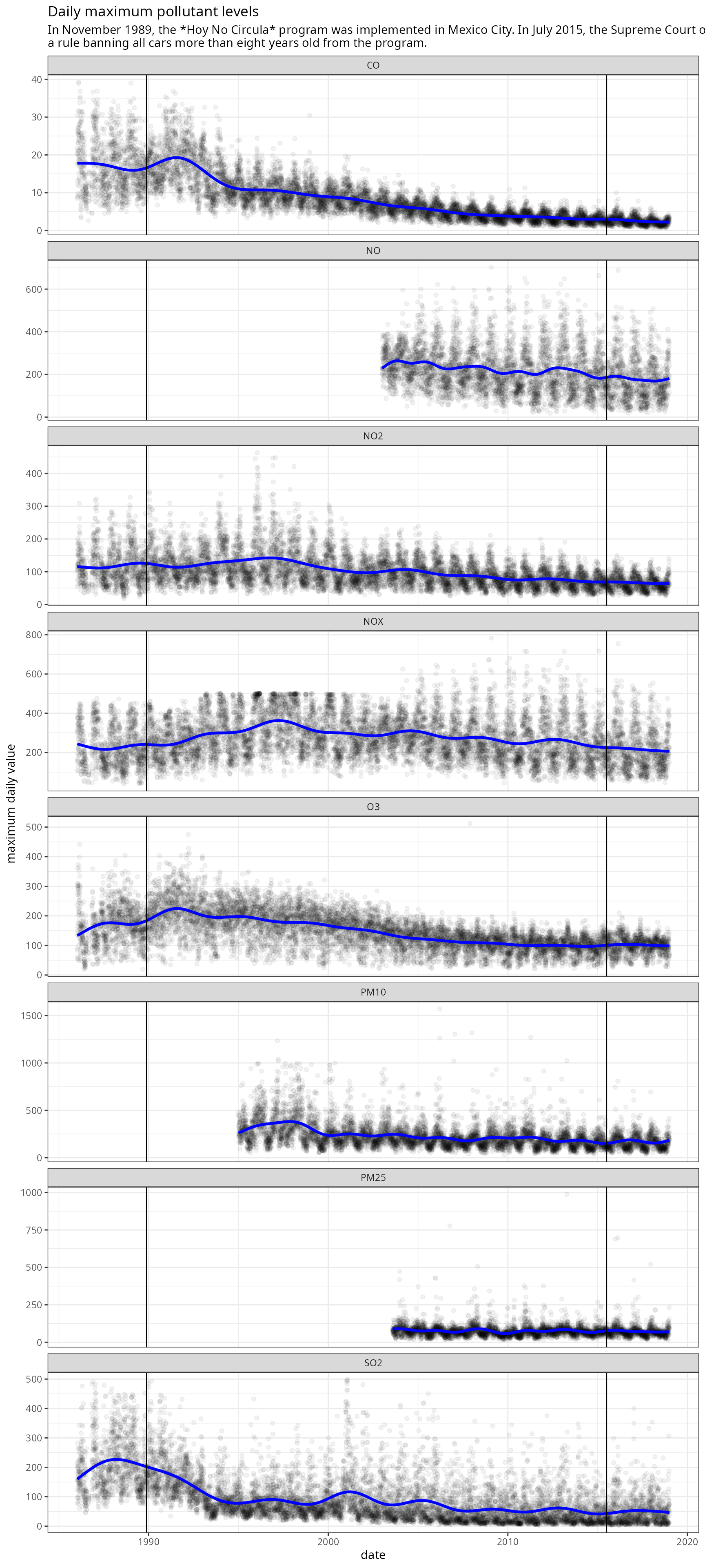
We can plot all pollutants going back to 1986 and add a trend line based on a GAM controlling for the month of the year. The plot includes vertical lines representing the start of Hoy No Circula and the Supreme Court decision that the program does not necessarily apply to older cars. A more complex model is left as an exercise for the reader.

fitted <- function(max, month, date, year) {
  df=data.frame(max = max,
                month = month,
                date = date,
                year = year)
  fit <- gam(max ~ s(month, bs = "cc", k = 12) + s(as.numeric(date), k = 20),
         data = df, correlation = corARMA(form = ~ 1|year, p = 1))
  predict(fit, newdata = df, type = "terms")[,2] + mean(max)
}
print("test")

## [1] "test"

df_maximos <- df_maximos %>%
  mutate(month = month(date),
         year = year(date))%>%
  group_by(pollutant) %>%
  mutate(pred = fitted(max,month,date,year)) %>%
  ungroup()
print("test2")

## [1] "test2"

# Plot the daily highest level with trendline
ggplot(df_maximos, 
       aes(date, max, group = 1)) +
  geom_point(color = "black", linewidth = .2, alpha = .05) +
  geom_line(aes(date, pred), color ="blue", linewidth = 1.2)  +
  labs(title = "Daily maximum pollutant levels",
       subtitle = "In November 1989, the *Hoy No Circula* program was implemented in Mexico City. In July 2015, the Supreme Court overturned\na rule banning all cars more than eight years old from the program.") +
  ylab("maximum daily value") +
  xlab("date") +
  geom_vline(xintercept = as.Date("1989-11-20")) +
  geom_vline(xintercept = as.Date("2015-07-01")) +
  theme_bw() +
  facet_wrap(~pollutant, scales = "free_y", ncol = 1)

## Warning in geom_point(color = "black", linewidth = 0.2, alpha = 0.05):
## Ignoring unknown parameters: `linewidth`