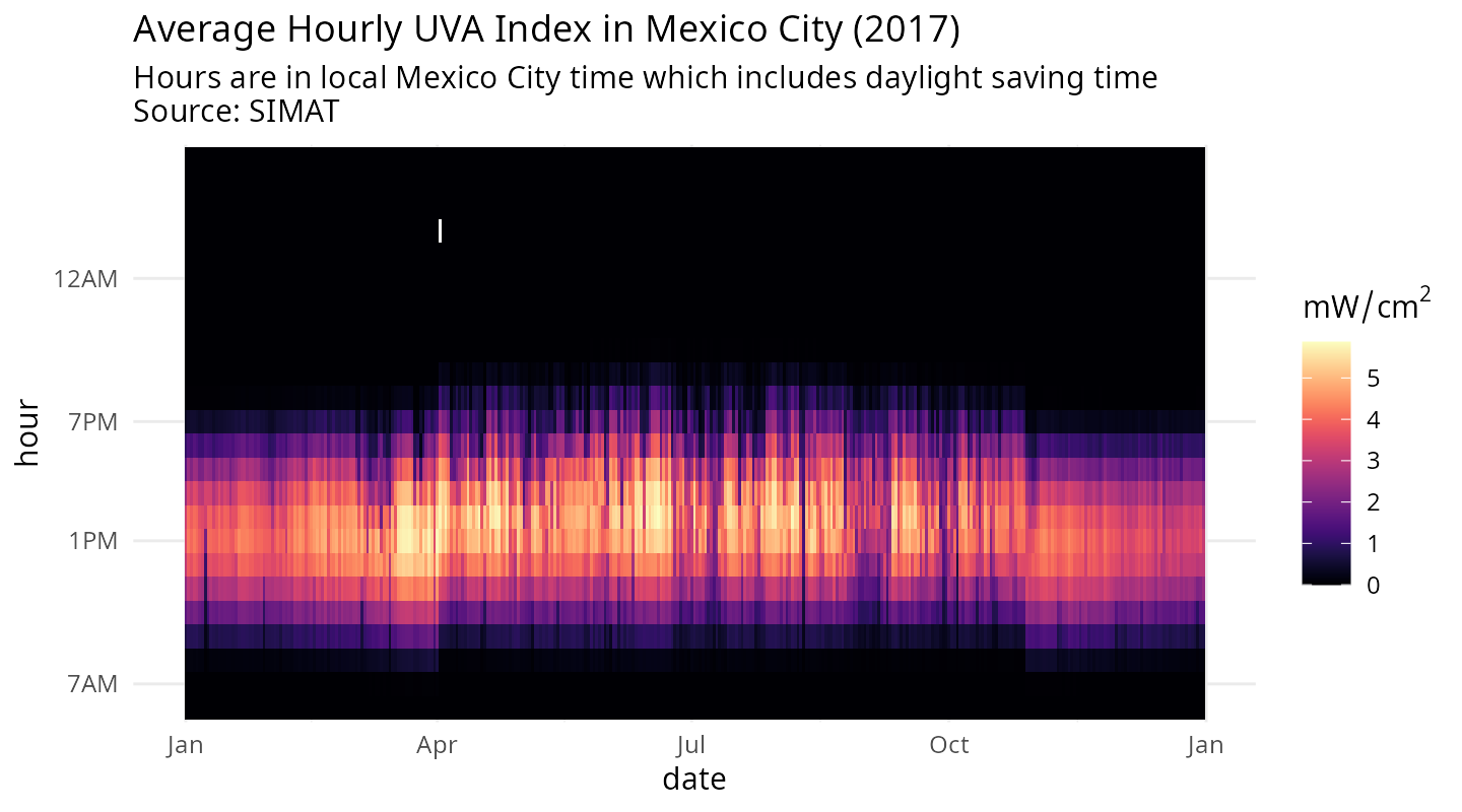
This document visualizes the average hourly Ultraviolet A (UVA) radiation levels across Mexico City throughout 2017. The data, provided by the Mexico City Air Quality Monitoring Network (SIMAT), illustrates seasonal and daily variations in exposure.
Notably, at the time of these measurements in 2017, Mexico City still observed Daylight Savings Time (DST). Consequently, the local time reflected in this visualization accounts for these seasonal clock shifts.
## Auto-install required R packages
if (!require("pacman")) install.packages("pacman")
pacman::p_load(aire.zmvm, dplyr, ggplot2, lubridate, viridis, scales)
df <- download_radiation(type = "UVA", 2017)
df$mxc_time <- format(as.POSIXct(paste0(df$date, " ", df$hour, ":00"),
                                 tz = "Etc/GMT+6"),
                      tz = "America/Mexico_City")
df$hour_mxc <- hour(df$mxc_time)
df <- df %>%
  group_by(date, hour_mxc) %>%
  summarise(mean = mean(value, na.rm = TRUE))
#> `summarise()` has regrouped the output.
#> ℹ Summaries were computed grouped by date and hour_mxc.
#> ℹ Output is grouped by date.
#> ℹ Use `summarise(.groups = "drop_last")` to silence this message.
#> ℹ Use `summarise(.by = c(date, hour_mxc))` for per-operation grouping
#>   (`?dplyr::dplyr_by`) instead.


df$year <- year(df$date)
df$yday <- yday(df$date)
df$day <- day(df$date)
df$month <- month(df$date)
df$hour_mxc <- factor(df$hour_mxc, levels = c(6:23,0:5))

ggplot(filter(df), aes(date, hour_mxc)) +
  geom_tile(aes(fill = mean)) +
  scale_fill_viridis(expression(mW/cm^{2}), option = "A") +
  scale_x_date(labels = date_format("%b")) +
  scale_y_discrete(breaks = c(7, 13, 18, 0),
                   labels = c("7AM", "1PM",  "7PM", "12AM")) +
  ggtitle("Average Hourly UVA Index in Mexico City (2017)",
          subtitle = "Hours are in local Mexico City time which includes daylight saving time\nSource: SIMAT") +
  theme_bw() +
  ylab("hour") +
  theme_minimal()