Ridge plot of January temperatures

Install the necessary packages:

# based on https://cran.r-project.org/web/packages/ggjoy/vignettes/gallery.html
## Auto-install required R packages
if (!require("pacman")) install.packages("pacman")
pacman::p_load(aire.zmvm, dplyr, ggplot2, tidyr, viridis, stringr, lubridate,
               ggridges, purrrlyr)

Download the data:

# Download January TMP from 2005 to 2008
# You could get TMP data accurate to one digit by using get_station_data,
# but there's no data for 2018 that way
temp <- data.frame()
for (year in 2005:2018) {
  df2 <- get_station_month_data("HORARIOS", "TMP", year, 1)
  temp <- rbind(temp, df2)
}

Clean the data and only use stations that were reporting 99% of the time during the period under analysis.

# remove stations that always report 0
temp <- temp %>%
  mutate(year = year(temp$date)) %>%
  group_by(year, station_code) %>%
  filter(!sum(value, na.rm = TRUE) == 0) %>%
  ungroup()

# Which stations reported a temperature value at least 99% of the time
reporting_stations_99 <- temp %>%
  group_by(year = year(date), station_code) %>%
  summarise(per = sum(!is.na(value)) / length(station_code)) %>%
  filter(per > .99) %>%
  select(year, station_code)  %>%
  slice_rows("year") %>%
  by_slice(function(x) unname(unlist(x)), .to = "vec")

# Subset only those stations that reported 99% of the time from 
# 2005 to 2018
temp <- filter(temp,
               station_code %in% unique(do.call(c, reporting_stations_99[[2]])))
print(unique(do.call(c, reporting_stations_99[[2]])))

##  [1] "CES" "MON" "PED" "PLA" "TLA" "VIF" "XAL" "FAC" "MER" "TAC" "TAH" "TPN"
## [13] "CUA" "SAG" "IMP" "ACO" "SUR" "SFE" "CHO" "CUT" "AJM" "MGH" "NEZ" "SS1"
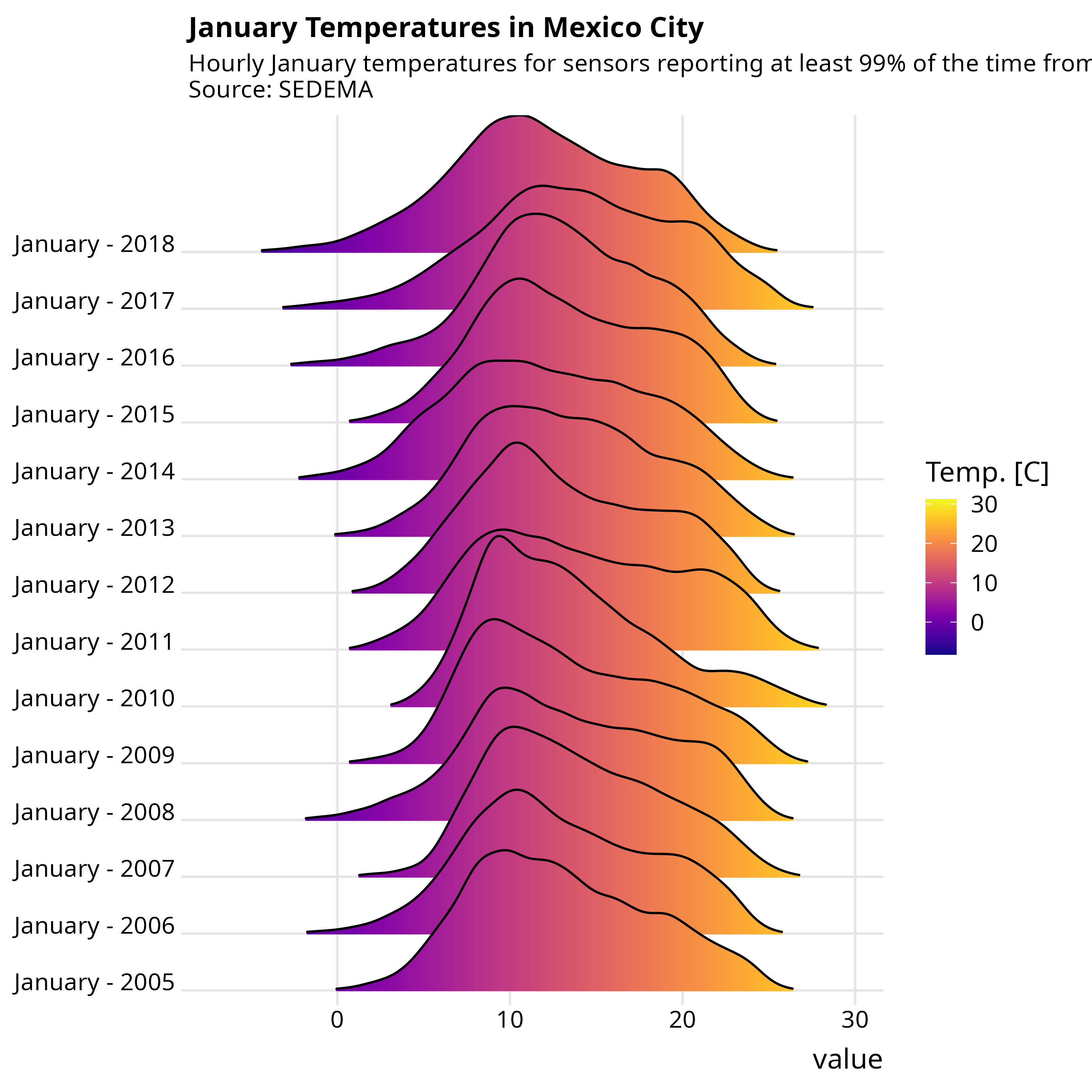
## [25] "UAX" "UIZ" "AJU" "MPA" "BJU"

Finally, we plot the data:

temp$month <- months(temp$date)
temp$month <- factor(temp$month, levels = rev(unique(temp$month)) )
temp$month <- str_c(temp$month, " - ", year(temp$date))

ggplot(temp, aes(x = value, y = month, fill = ..x..)) +
  geom_density_ridges_gradient(scale = 3, rel_min_height = 0.01, gradient_lwd = 1.) +
  scale_x_continuous(expand = c(0.01, 0)) +
  scale_y_discrete(expand = c(0.01, 0)) +
  scale_fill_viridis(name = "Temp. [C]", option = "C") +
  labs(title = 'January Temperatures in Mexico City',
       subtitle = paste0('Hourly January temperatures for sensors reporting ',
                         'at least 99% of the time from 2005 to ',
                         '2018\nSource: SEDEMA')) +
  theme_ridges(font_size = 13, grid = TRUE) + theme(axis.title.y = element_blank())

## Warning: The dot-dot notation (`..x..`) was deprecated in ggplot2 3.4.0.
## ℹ Please use `after_stat(x)` instead.
## This warning is displayed once per session.
## Call `lifecycle::last_lifecycle_warnings()` to see where this warning was
## generated.

## Picking joint bandwidth of 0.746