Pollutant levels, by hour

Here’s an example of plotting the maximum pollution value for Ozone and PM10, by hour of day. First we load the package necessary for performing the analysis:

## Auto-install required R packages
if (!require("pacman")) install.packages("pacman")
pacman::p_load(aire.zmvm, dplyr, ggplot2, lubridate, stringr)

Once loaded, we can download O₃ and PM_10M data in the original units using the get_station_data function:

download_horarios <- function(pollutant) {
  #print(paste0("Downloading data for: ", pollutant))
  df <- get_station_data(criterion = "HORARIOS", # Can be MAXIMOS (daily maximum), 
                         # MINIMOS (daily minimum), 
                         # or HORARIOS (hourly average)
                         pollutant = pollutant, # "SO2", "CO", "NOX", "NO2", "NO", "O3", 
                         # "PM10", "PM25", "WSP", "WDR", "TMP", "RH"
                         year = 2007:2017) # The earliest year allowed is 1986
  df$pollutant <- pollutant
  # Daily max among all base stations
  df %>% 
    group_by(date, hour, pollutant) %>% 
    summarise(max = ifelse(all(is.na(value)),
                           NA,
                           base::max(value, na.rm = TRUE))) %>%
    na.omit() %>%
    ungroup()
}

ll_horarios <- mapply(download_horarios, 
                      pollutant = c("O3", "PM10"),
                      SIMPLIFY = FALSE)

## `summarise()` has regrouped the output.
## `summarise()` has regrouped the output.
## ℹ Summaries were computed grouped by date, hour, and pollutant.
## ℹ Output is grouped by date and hour.
## ℹ Use `summarise(.groups = "drop_last")` to silence this message.
## ℹ Use `summarise(.by = c(date, hour, pollutant))` for per-operation grouping
##   (`?dplyr::dplyr_by`) instead.

df_horarios <- bind_rows(ll_horarios)

Dealing with daylight savings time

The data returned by get_station_data when using the “HORARIOS” criterion includes the date and hour of each measurement. The hour is specified as an offset from midnight and does not include daylight saving time (effectively GMT+6). It is advisable to convert this to local Mexico City time if we want to analyze pollution patterns by hour of day.

knitr::kable(head(df_horarios))

date	hour	pollutant	max
2007-01-01	1	O3	11
2007-01-01	2	O3	10
2007-01-01	3	O3	12
2007-01-01	4	O3	13
2007-01-01	5	O3	15
2007-01-01	6	O3	14

# The time is given in hours with no DST
# GMT has no DST
df_horarios$datetime <- as.POSIXct(
  strptime(paste0(df_horarios$date, " ", df_horarios$hour),
           "%Y-%m-%d %H", tz = "Etc/GMT+6")
)
# Convert to MXC time
df_horarios$datetime_mxc <- as.POSIXct(format(df_horarios$datetime, 
                                          tz="America/Mexico_City",
                                          usetz = TRUE))
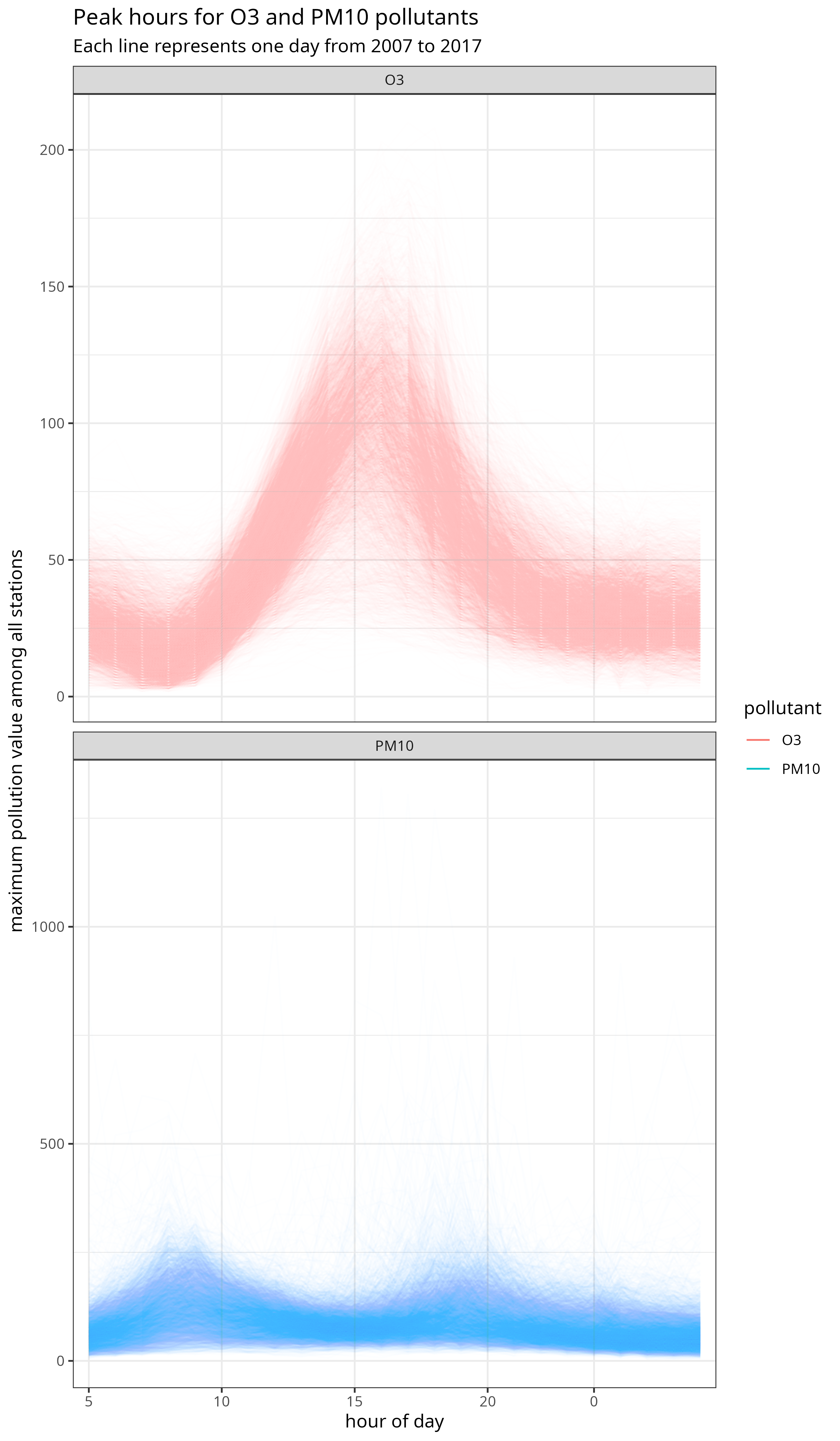
df_horarios$hour_dst <- hour(df_horarios$datetime_mxc)

Ozone peaks a couple of hours after midday, while PM10 particles peak during commuting hours (according to the Encuesta Origen-Destino 2017), and also sometimes around midnight due to fireworks and trash burning. A Phase I contingency is declared when the 24-hour average PM10 concentration exceeds 150 IMECAs in at least two stations, and for O3 when the hourly average exceeds 150 IMECAs (data is shown in the original units, not IMECAs).

df_horarios$hour_dst <- factor(df_horarios$hour_dst, 
                               levels = c(5:23, 0:4), 
                               ordered = TRUE)

ggplot(df_horarios, 
       aes(hour_dst, max, group = date, color = pollutant)) +
  geom_line(alpha = I(1/sqrt((2017-2001)*1565))) +
  facet_wrap(~pollutant, scales = "free_y", ncol = 1) +
  guides(color = guide_legend("pollutant",
                              override.aes = list(alpha = 1))) +
  theme_bw() +
  xlab("hour of day") +
  ylab("maximum pollution value among all stations") +
  scale_x_discrete(breaks = seq(0, 23, 5)) +
  labs(title = "Peak hours for O3 and PM10 pollutants",
       subtitle = "Each line represents one day from 2007 to 2017")