![]()

aire.zmvm is an R package for downloading air quality data from the Mexico City metropolitan area. This package provides real-time, daily maximum, minimum, and hourly average data for pollution measuring stations and geographical zones within the Zona Metropolitana del Valle de México (Greater Mexico City). It also includes station locations and a specialized function for inverse distance weighting adjusted for wind direction.
Installation
You can always install the development version from GitHub:
if (!require(devtools)) {
    install.packages("devtools")
}
devtools::install_github('diegovalle/aire.zmvm')
To install the stable version from CRAN, use:
install.packages("aire.zmvm")
library(aire.zmvm)
Note: The version on CRAN may not include the latest updates available on GitHub.
Usage
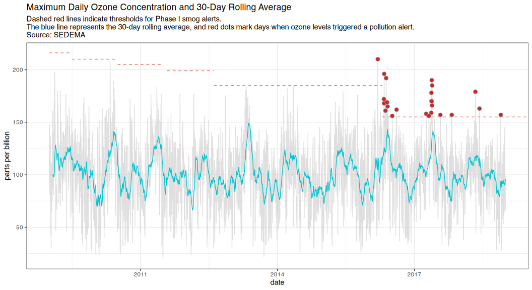
This example creates a time series of ozone levels (in ppb) from 2009 to 2018 and highlights Phase I smog alerts.
# Automatically install and load required packages
if (!require("pacman")) install.packages("pacman")
pacman::p_load(aire.zmvm, dplyr, ggplot2, ggseas)

# Download pollution data by station (in ppb)
o3 <- get_station_data(criterion = "MAXIMOS", # Can be one of MAXIMOS (maximum),
                                              # MINIMOS (minimum),
                                              # or HORARIOS (hourly average)
                       pollutant = "O3", # Can be one of "SO2", "CO", "NOX",
                                         # "NO2", "NO", "O3", "PM10", "PM25",
                                         #  "WSP", "WDR", "TMP", "RH"
                       year = 2009:2018) # A numeric vector, the earliest #
                                         # year allowed is 1986
# Daily max among all base stations
o3_max <- o3 %>%
  group_by(date) %>%
  summarise(max = ifelse(all(is.na(value)),
                         NA,
                         base::max(value, na.rm = TRUE))) %>%
  na.omit()

# Ozone thresholds for declaring a 'smog alert' and their periods of validity
# source:
# http://www.aire.cdmx.gob.mx/descargas/ultima-hora/calidad-aire/pcaa/pcaa-modificaciones.pdf
contingencia_levels <- data.frame(
  ppb = c(216, 210, 205,
          199, 185, 155, 155),
  start = c(2009, 2009.4973, 2010.4973, 2011.5795,
            2012.6052,  2016.291, 2016.4986),
  end = c(2009.4973, 2010.4945, 2011.4945,
          2012.6025,    2016.2883, 2016.4959, Inf))
max_daily_df <- tsdf(ts(o3_max$max, start = c(2009,1), frequency = 365.25))

contingencia <- o3_max
contingencia$date <- max_daily_df$x
contingencia$contingencia <- case_when(
  contingencia$date > 2012.6052 & contingencia$max > 185 ~ TRUE,
  contingencia$date > 2016.291 & contingencia$max > 155 ~ TRUE,
  TRUE ~ FALSE
)
Below is a preview of the downloaded data:
| date | station_code | pollutant | unit | value |
|---|---|---|---|---|
| 2009-01-01 | ACO | O3 | ppb | 67 |
| 2009-01-02 | ACO | O3 | ppb | 71 |
| 2009-01-03 | ACO | O3 | ppb | 112 |
| 2009-01-04 | ACO | O3 | ppb | 91 |
| 2009-01-05 | ACO | O3 | ppb | 70 |
| 2009-01-06 | ACO | O3 | ppb | 71 |
ggplot(max_daily_df,
       aes(x = x, y = y)) +
  geom_line(colour = "grey75", alpha = .5) +
  stat_rollapplyr(width = 30, align = "right", color = "#01C5D2") +
  geom_segment(data = contingencia_levels,
               aes(x=start, y=ppb, xend=end, yend=ppb), color="#E3735E",
               linetype = 2)  +
  geom_point(data=filter(contingencia, contingencia == TRUE),
             aes(x=date, y=max), color = "#999999",
             size = 2.5, shape = 21, fill = "firebrick3" ) +
  xlab("date") +
  ylab("parts per billion") +
  scale_x_continuous(breaks = c(2011, 2014, 2017)) +
  ggtitle("Maximum Daily Ozone Concentration and 30-Day Rolling Average",
          subtitle = paste0("Dashed red lines indicate thresholds for ",
                            "Phase I smog alerts. \nThe blue line represents ",
                            "the 30-day rolling average, and red dots mark ",
                            "days when ozone levels triggered a pollution alert.\n",
                            "Source: SEDEMA")) +
  theme_bw()