Comparing rsinaica to aire.zmvm

This vignette compares air quality data retrieved via the rsinaica package against data from the aire.zmvm package. To ensure a fair comparison, we will analyze Ozone (O₃) levels from the Xalostoc station in Mexico City for the same time period.

Load Required Packages

First, we load the necessary libraries for data manipulation, visualization, and API access:

## Auto-install required R packages
packs <- c("dplyr", "ggplot2", "lubridate", "aire.zmvm", "rsinaica")
load_pkg <- function(pkg) {
  suppressWarnings(require(pkg, character.only = TRUE))
}
success <- vapply(packs, load_pkg, logical(1))
missing <- packs[!success]
if (length(missing)) {
  install.packages(missing)
  vapply(missing, load_pkg, logical(1))
}

The hourly data from the aire.zmvm package generally use the GMT+6 time zone (with no Daylight Saving Time). In contrast, according to the stations_sinaica data.frame, data for the Xalostoc station is recorded in local Mexico City time, which included Daylight Saving Time in the summer it was collected. Please note that each station submits its data to SINAICA using its preferred time zone, and the reported time zone may occasionally be incorrect.

## 271 is the station_id of Xalostoc
stations_sinaica$timezone[stations_sinaica$station_id == 271]
#> [1] "Tiempo del centro, UTC-6 (UTC-5 en verano)"

Next, we download the data and ensure that values from both aire.zmvm and rsinaica are in parts per billion (ppb). Since rsinaica returns values in parts per million (ppm), we multiply them by 1,000.

df_aire <- get_station_month_data("HORARIOS", "O3", 2017, 5) %>%
  filter(station_code == "XAL") %>%
  mutate(value_aire.zmvm = value)
## data from get_station_month_data is in GMT+6
df_aire$datetime <-  as.POSIXct(
  strptime(paste0(df_aire$date, " ", df_aire$hour),
           "%Y-%m-%d %H", tz = "Etc/GMT+6")
)
df_aire <- df_aire[, c("datetime", "value_aire.zmvm")]


## values from sinaica are in ppb and those from aire.zmvm in ppm
## Xalostoc station has an rsinaica station_id of 271
df_sinaica <- sinaica_station_data(271, "O3", "2017-05-01", "2017-05-31") %>%
  mutate(value = value * 1000) %>%
  mutate(value_sinaica = value) %>%
  mutate(date = as.Date(date))
## data from rsinaica is in the local Mexico City time zone
df_sinaica$datetime <-  as.POSIXct(
  strptime(paste0(df_sinaica$date, " ", df_sinaica$hour),
           "%Y-%m-%d %H", tz = "America/Mexico_City")
)
df_sinaica <- df_sinaica[, c("datetime", "value_sinaica")]

df <- full_join(df_aire, df_sinaica, by = c("datetime" = "datetime"))

The merged data is shown below:

	datetime	value_aire.zmvm	value_sinaica
5	2017-05-01 05:00:00	2	2
6	2017-05-01 06:00:00	2	2
7	2017-05-01 07:00:00	3	3
8	2017-05-01 08:00:00	5	5
9	2017-05-01 09:00:00	17	17
10	2017-05-01 10:00:00	55	55

The mean squared error is as follows:

mean((df$value_aire.zmvm - df$value_sinaica)^2, na.rm = TRUE)
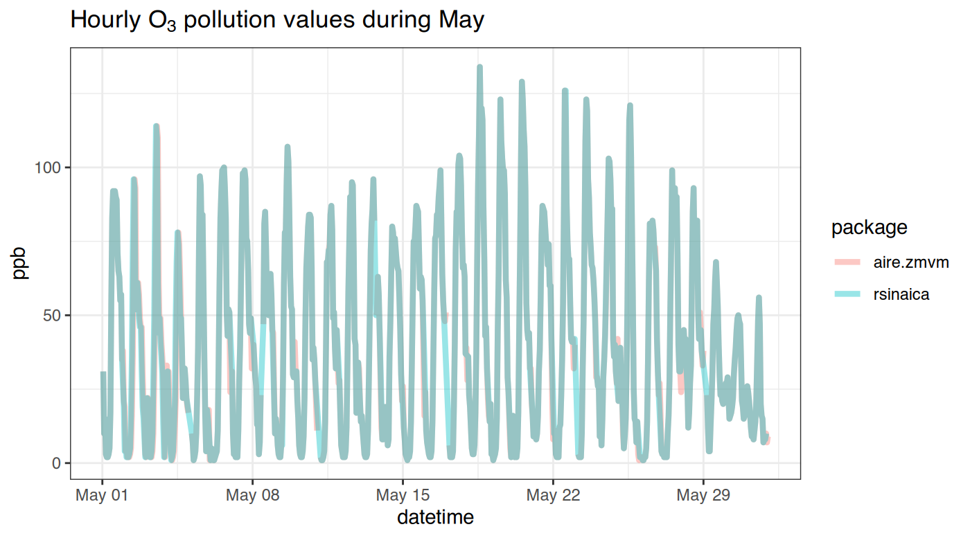
#> [1] 22.01807

We can visually compare them with a plot. The values are extremely similar, but the aire.zmvm data is slightly more accurate since it comes directly from the source.

ggplot(df_aire, aes(datetime, value_aire.zmvm, color = "aire.zmvm")) +
  geom_line(size = 1.5, alpha = .4) +
  geom_line(data = df_sinaica, aes(datetime, value_sinaica, color = "rsinaica"),
            alpha = .4, size = 1.5) +
  xlab("datetime") +
  ylab("ppb") +
  scale_color_discrete("package") +
  ggtitle(expression(paste("Hourly ", 
                           O[3], 
                           " pollution values during May"))) +
  theme_bw()
#> Warning: Using `size` aesthetic for lines was deprecated in ggplot2 3.4.0.
#> ℹ Please use `linewidth` instead.
#> This warning is displayed once per session.
#> Call `lifecycle::last_lifecycle_warnings()` to see where this warning was
#> generated.

Diego Valle-Jones

2026-03-06

Load Required Packages