![]()

![]()
| Author: | Diego Valle-Jones |
| License: | MIT + file LICENSE |
| Website: | https://hoyodesmog.diegovalle.net/rsinaica/ |
| Help: | https://github.com/diegovalle/rsinaica/discussions |
Easy-to-use functions for downloading air quality data from the Mexican National Air Quality Information System (SINAICA). This R package allows you to download pollution and meteorological data from more than one hundred monitoring stations across Mexico. You can query crude real-time data, validated data, or manually collected data.
Installation
To install the most recent package version from CRAN, run:
install.packages("rsinaica")You can always install the development version from GitHub:
if (!require(devtools)) {
    install.packages("devtools")
}
devtools::install_github("diegovalle/rsinaica")
Example
Suppose you want to download pollution data from the Centro station in Guadalajara. First, load the required packages and look up the station’s numeric code in the stations_sinaica data.frame:
## Auto-install required R packages
packs <- c("ggplot2", "maps", "mapproj", "rsinaica")
success <- suppressWarnings(sapply(packs, require, character.only = TRUE))
if (length(names(success)[!success])) {
  install.packages(names(success)[!success])
  sapply(names(success)[!success], require, character.only = TRUE)
}

knitr::kable(stations_sinaica[
  which(stations_sinaica$station_name == "Centro"),  1:6
])| station_id | station_name | station_code | network_id | network_name | network_code | |
|---|---|---|---|---|---|---|
| 28 | 33 | Centro | CEN | 30 | Aguascalientes | AGS |
| 29 | 54 | Centro | CEN | 38 | Chihuahua | CHIH1 |
| 30 | 102 | Centro | CEN | 63 | Guadalajara | GDL |
| 31 | 170 | Centro | CEN | 78 | Zona Metropolitana de Querétaro | ZMQ |
There are three stations named Centro. The one we want is located in Guadalajara and has a numeric code (station_id) of 102. The stations_sinaica data.frame also includes the latitude and longitude of all monitoring stations in Mexico (including some that have never reported data)..
mx <- map_data("world", "Mexico")
stations_sinaica$color <- "Others"
stations_sinaica$color[stations_sinaica$station_id == 102] <- "Centro (102)"
## There seems to be a mistake in some of the air quality stations longitudes
## having been assigned positive values (longitudes to the west of the
## prime meridian are supposed to be negative)
stations_sinaica <- subset(stations_sinaica, lon < 0)
ggplot(stations_sinaica[order(stations_sinaica$color, decreasing = TRUE),],
       aes(lon, lat)) +
  geom_polygon(data = mx, aes(x= long, y = lat, group = group)) +
  geom_point(alpha = .9, size = 3, aes(fill = color), shape = 21) +
  scale_fill_discrete("station") +
  ggtitle("Air quality measuring stations in Mexico") +
  coord_map() +
  theme_void()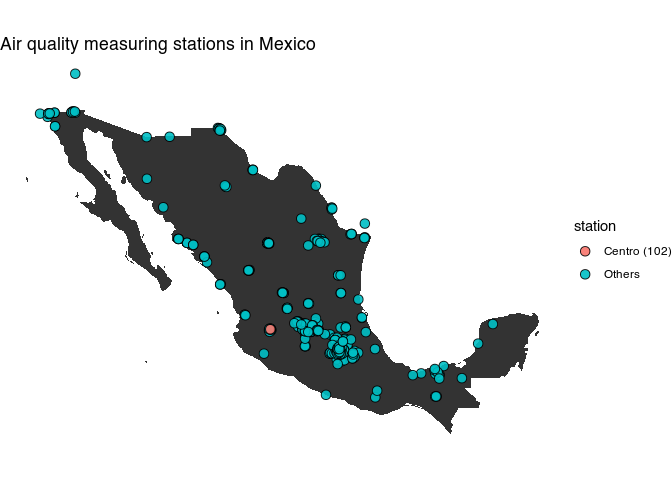
Next, query the start and end dates for which SINAICA has received data from this station:
sinaica_station_dates(102)
#> [1] "1997-01-01" "2026-06-01"
The station is currently reporting data (this document was built on 2026-06-01), and it has been active since 1997. You can also query which parameters (pollution, wind, solar radiation, etc.) the station measures. the station has sensors for. The package also includes a parameters data.frame containing the complete set of supported parameters; however, not all stations report all of them.
cen_params <- sinaica_station_params(102)
knitr::kable(cen_params)| param_code | param_name |
|---|---|
| CN | Carbono negro |
| SO2 | Dióxido de azufre |
| NO2 | Dióxido de nitrógeno |
| DV | Dirección del viento |
| HR | Humedad relativa |
| IUV | Índice de radiación ultravioleta |
| CO | Monóxido de carbono |
| NO | Óxido nítrico |
| NOx | Óxidos de nitrógeno |
| O3 | Ozono |
| PM10 | Partículas menores a 10 micras |
| PM2.5 | Partículas menores a 2.5 micras |
| PP | Precipitación pluvial |
| PB | Presión Barométrica |
| RS | Radiación solar |
| TMP | Temperatura |
| TMPI | Temperatura interior |
| VV | Velocidad del viento |
Finally, download and plot hourly concentrations of particulate matter with a diameter smaller than 10 micrometers (μm) (PM10), for the month of January.
# Download all PM10 data for January 2018
df <-  sinaica_station_data(102, # station_id
                         "PM10", # parameter
                         "2018-01-01", # start_date
                         "2018-01-31", # end_date
                         "Crude" # Crude, Manual or Validated
                         )

ggplot(df, aes(hour, value, group = date)) +
  geom_line(alpha=.9) +
  ggtitle(expression(paste(PM[10],
                           " pollution during January 2018 at the",
                           " Centro station in Guadalajara"))) +
  labs(subtitle="Each line corresponds to a day") +
  xlab("hour") +
  ylab(expression(paste(mu,"g/", m^3))) +
  theme_bw()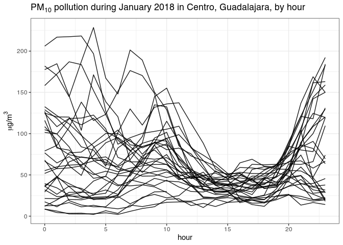
The hours are shown in the local Guadalajara time zone (UTC−6), since we plotted January 2018 data.
stations_sinaica$timezone[which(stations_sinaica$station_id == 102)]
#> [1] "Tiempo del centro, UTC-6 (UTC-5 en verano)"
You can find a handy map of Mexico’s time zones from Wikipedia to help you with any time conversions you might need.