We can use the idw360 function to extrapolate wind direction and speed inside a grid. First we load the packages:
## Auto-install required R packages
if (!require("pacman")) install.packages("pacman")
pacman::p_load(aire.zmvm, dplyr, ggplot2, lubridate, stringr, sp, mapproj,
               gstat, ggmap)
and then download the wind speed and direction data
# download wind speed and direction and filter March 28, 2018 7:00 PM
wsp <- get_station_month_data(criterion = "HORARIOS",
                              pollutant = "WSP",
                              2018, 3)%>%
  filter(date == "2018-03-28" & hour == 19) %>%
  na.omit()
wdr <- get_station_month_data(criterion = "HORARIOS",
                        pollutant = "WDR",
                        year = 2018, 3) %>%
  filter(date == "2018-03-28" & hour == 19)  %>%
  na.omit()
This is what the data look like
| date | hour | station_code | pollutant | unit | value | |
|---|---|---|---|---|---|---|
| 2 | 2018-03-28 | 19 | AJM | WSP | m/s | 10.2 |
| 5 | 2018-03-28 | 19 | BJU | WSP | m/s | 4.6 |
| 9 | 2018-03-28 | 19 | MON | WSP | m/s | 6.5 |
| 10 | 2018-03-28 | 19 | CHO | WSP | m/s | 3.5 |
| 12 | 2018-03-28 | 19 | CUA | WSP | m/s | 4.3 |
| 14 | 2018-03-28 | 19 | FAC | WSP | m/s | 3.8 |
| date | hour | station_code | pollutant | unit | value | |
|---|---|---|---|---|---|---|
| 2 | 2018-03-28 | 19 | AJM | WDR | ° | 198 |
| 5 | 2018-03-28 | 19 | BJU | WDR | ° | 169 |
| 9 | 2018-03-28 | 19 | MON | WDR | ° | 165 |
| 10 | 2018-03-28 | 19 | CHO | WDR | ° | 150 |
| 12 | 2018-03-28 | 19 | CUA | WDR | ° | 246 |
| 14 | 2018-03-28 | 19 | FAC | WDR | ° | 205 |
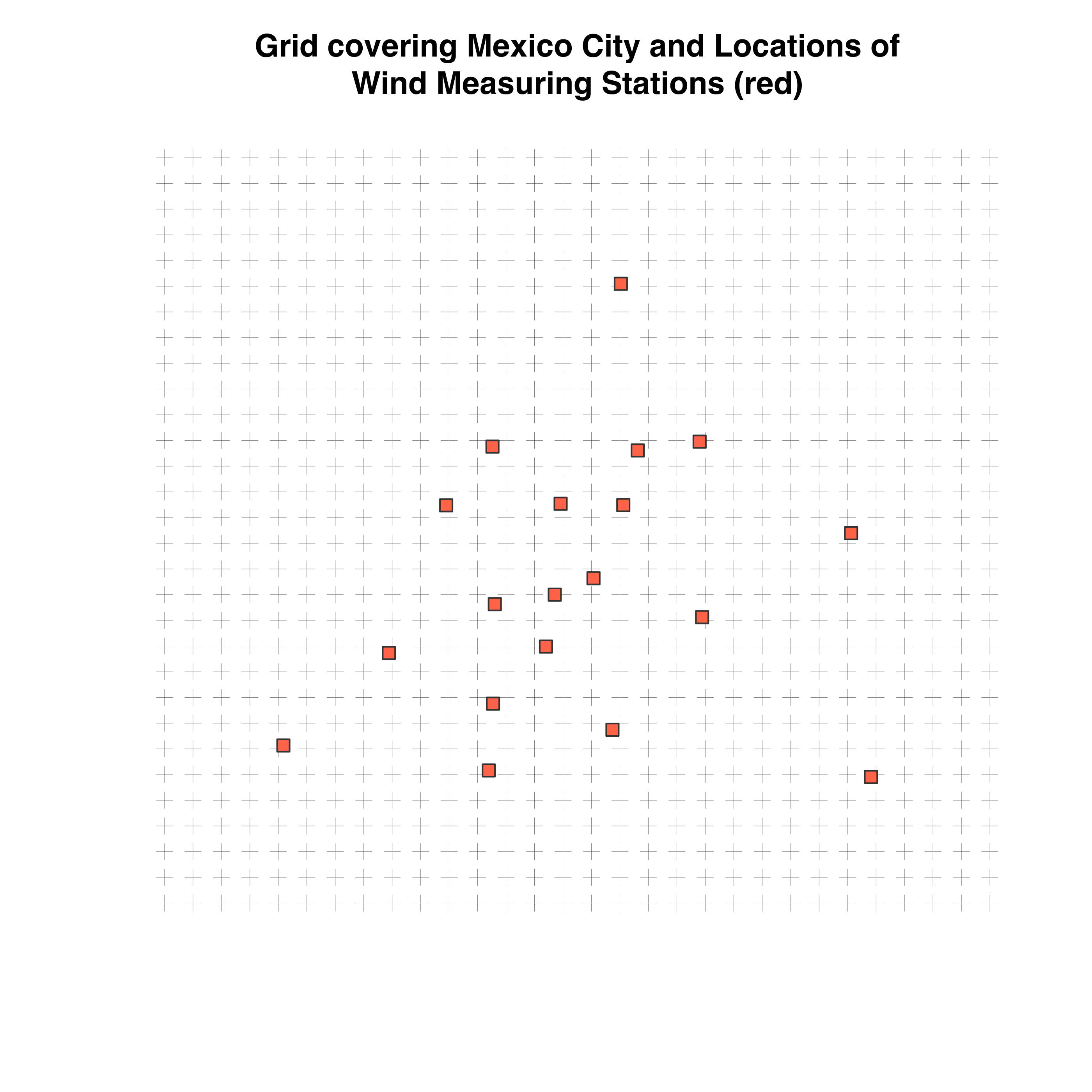
| We ca | n create a po | int gri | d over which to | extrapolate | the wi | nd values |
## Location of sensors. First column x/longitude, second y/latitude
locations <- stations[, c("station_code", "lon", "lat")]
locations <- merge(wdr, locations)
coordinates(locations) <- ~lon+lat
proj4string(locations) <- CRS("+proj=longlat +ellps=WGS84 +no_defs +towgs84=0,0,0")

## The grid for which to extrapolate values
pixels = 30
grid <- expand.grid(lon = seq((min(coordinates(locations)[, 1]) - .1),
                              (max(coordinates(locations)[, 1]) + .1),
                              length.out = pixels),
                    lat = seq((min(coordinates(locations)[, 2]) - .1),
                              (max(coordinates(locations)[, 2]) + .1),
                              length.out = pixels))
grid<- SpatialPoints(grid)
proj4string(grid) <- CRS("+proj=longlat +ellps=WGS84 +no_defs +towgs84=0,0,0")

plot(grid, main = "Grid covering Mexico City and Locations of\nWind Measuring Stations (red)",
     col = "#666666", lwd = .2)
# Plot the locations of the stations
geog <- stations[stations$station_code %in% unique(wsp$station_code), c("lat", "lon")]
coordinates(geog) <- ~lon+lat
points(geog, pch = 22, col = "#333333", bg = "tomato1", cex = 1.2)
extrapolate using inverse distance weighting
# extrapolate wind direction
res <- idw360(wdr$value, locations, grid)

# extrapolate wind speed
wsp <- left_join(wsp, stations, by = "station_code")
wsp <- wsp[!is.na(wsp$value),]
wsp <- wsp[,c("lat", "lon", "value")]
coordinates(wsp) <- ~lon+lat
proj4string(wsp) <- CRS("+proj=longlat +ellps=WGS84 +no_defs +towgs84=0,0,0")
wsp <- idw(value ~ 1, wsp, grid, idp = 2, debug.level = 0)
wsp = as.data.frame(wsp)
names(wsp) <- c("lon", "lat", "var1.wsp", "var1.var")

# Combine wind direction and speed with the grid
df <- cbind(res, as.data.frame(grid), wsp = wsp$var1.wsp)
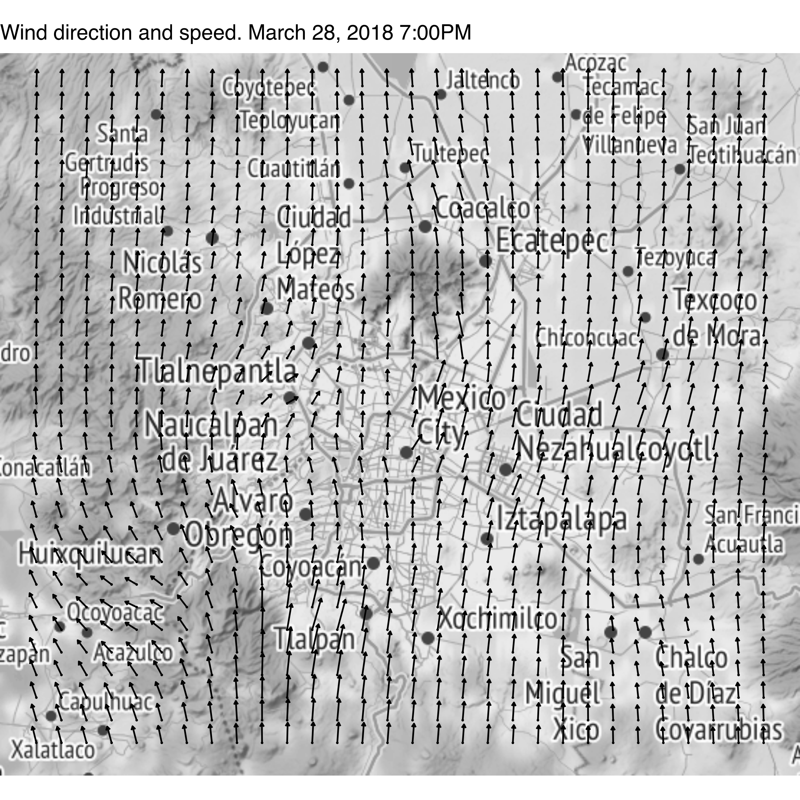
and finally we plot the data (Note that you may have to install a beta version of ggmap by running: devtools::install_github("dkahle/ggmap", ref = "tidyup"))
df$group <- 1
qmplot(lon, lat, data = df, geom = "blank",
       maptype = "toner-lite", source = "stamen",  zoom = 10, mapcolor = "bw") +
  geom_point(size = .1) +
  # The wind direction compass starts where the 90 degree mark is located
  geom_spoke(aes(angle = ((270 -  pred) %% 360) * pi / 180,
                 radius = wsp * .003),
             arrow = arrow(length = unit(0.09, "cm"))) +
  ggtitle("Wind direction and speed. March 28, 2018 7:00PM")