Load packages
## Auto-install required R packages
if (!require("pacman")) install.packages("pacman")
pacman::p_load(aire.zmvm, dplyr, ggplot2, lubridate, readr, stringr, mgcv)
Download the data
df <- download_deposition(deposition = "HUMEDO", type = "CONCENTRACION") %>%
  filter(pollutant == "PP")

# When does the SIMAT start recording rainfall each year?
knitr::kable(df %>%
        group_by(year(date)) %>%
        summarise(min = min(date)))
#> `summarise()` ungrouping output (override with `.groups` argument)
| year(date) | min |
|---|---|
| 1997 | 1997-05-05 |
| 1998 | 1998-05-04 |
| 1999 | 1999-02-22 |
| 2000 | 2000-02-14 |
| 2001 | 2001-01-08 |
| 2002 | 2002-02-04 |
| 2003 | 2003-05-05 |
| 2004 | 2004-05-03 |
| 2005 | 2005-05-09 |
| 2006 | 2006-05-08 |
| 2007 | 2007-04-30 |
| 2008 | 2008-05-05 |
| 2009 | 2009-05-11 |
| 2010 | 2010-05-03 |
| 2011 | 2011-05-02 |
| 2012 | 2012-05-07 |
| 2013 | 2013-04-29 |
| 2014 | 2014-04-28 |
| 2015 | 2015-05-04 |
| 2016 | 2016-05-02 |
| 2017 | 2017-05-08 |
| 2018 | 2018-04-23 |
| 2019 | 2019-04-22 |
Model with a GAM
# rainfall is measured around the begginig of may starting in May 2003
df <- df %>% filter(year(df$date) >= 2003)
df$week <- week(df$date)
df$year <- year(df$date)

# no measures of rainfall outside the rainy season, so set them to zero
df <- full_join(df,
          data.frame(
            year = year(seq(as.Date("2003-01-01"),
                            as.Date("2016-12-31"),
                            by = "week")),
            week = week(seq(as.Date("2003-01-01"),
                                as.Date("2016-12-31"),
                                by = "week"))
            ),
          by = c("year", "week")) %>%
  arrange(year, week)
df$value[is.na(df$value)] <- 0

df$date <- as.Date(str_c(df$year, "-", df$week,"-",1), format = "%Y-%U-%u")
#fit <- gam(value ~ te(as.numeric(date), week, bs = c("tp", "cc"), k = c(10, 52)),
#           data = df, family = nb())
#plot(fit, pers = TRUE)
fit2 <- gam(value ~ s(as.numeric(date)) + s(week), data = df, family = nb())

summary(fit2)
#>
#> Family: Negative Binomial(1.361)
#> Link function: log
#>
#> Formula:
#> value ~ s(as.numeric(date)) + s(week)
#>
#> Parametric coefficients:
#>             Estimate Std. Error z value Pr(>|z|)
#> (Intercept)   1.3158     0.3952    3.33 0.000869 ***
#> ---
#> Signif. codes:  0 '***' 0.001 '**' 0.01 '*' 0.05 '.' 0.1 ' ' 1
#>
#> Approximate significance of smooth terms:
#>                       edf Ref.df  Chi.sq  p-value
#> s(as.numeric(date)) 8.336  8.876   66.32 4.15e-11 ***
#> s(week)             8.013  8.102 1717.86  < 2e-16 ***
#> ---
#> Signif. codes:  0 '***' 0.001 '**' 0.01 '*' 0.05 '.' 0.1 ' ' 1
#>
#> R-sq.(adj) =  0.186   Deviance explained = 34.7%
#> -REML =  27624  Scale est. = 1         n = 6556
df$pred <- predict(fit2, newdata = df, type = "response")
Plots
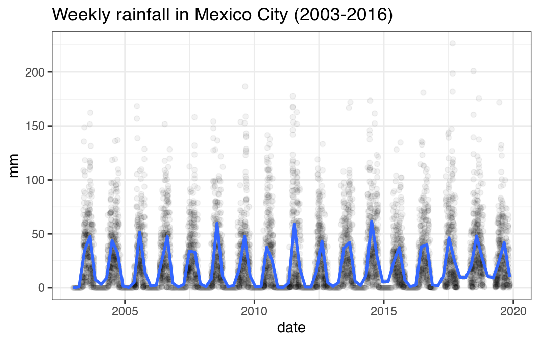
ggplot(df, aes(date, value)) +
  geom_point(alpha = .05) +
  geom_smooth(method = 'gam', formula = y ~ s(x, k = 53),
              method.args= list(family = nb())) +
  ggtitle("Weekly rainfall in Mexico City (2003-2016)") +
  ylab("mm") +
  theme_bw()
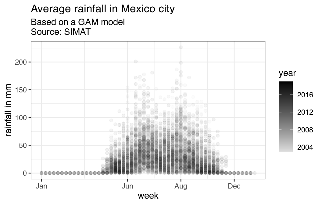
ggplot(df, aes(week, value, group = year, color = year)) +
  geom_point(alpha = .05) +
  ggtitle("Average rainfall in Mexico city",
          subtitle = "Based on a GAM model\nSource: SIMAT") +
  ylab("rainfall in mm") +
  scale_x_continuous(breaks = c(1,  week("2016-06-01"),
                                week("2016-09-01"), week("2016-12-01")),
                     labels = c("Jan", "Jun", "Aug", "Dec")) +
  scale_color_continuous(low="#dddddd", high = "black") +
  theme_bw()
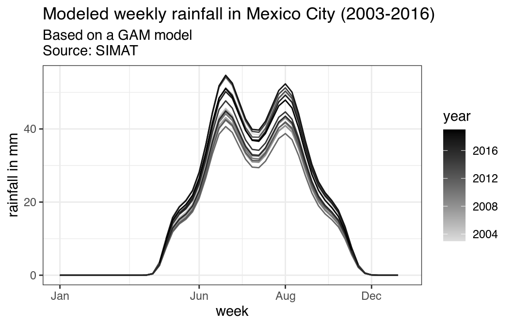
ggplot(df, aes(week, pred, group = year, color = year)) +
  geom_line() +
  ggtitle("Modeled weekly rainfall in Mexico City (2003-2016)",
          subtitle = "Based on a GAM model\nSource: SIMAT") +
  ylab("rainfall in mm") +
  scale_x_continuous(breaks = c(1,  week("2016-06-01"),
                                week("2016-09-01"), week("2016-12-01")),
                     labels = c("Jan", "Jun", "Aug", "Dec")) +
  scale_color_continuous(low="#dddddd", high = "black") +
  theme_bw()