Cold Weather School Closings

Because of low temperatures education authorities decided to suspend classes in public and private schools in some parts of Mexico City on Wednesday January 31, 2018. We will download and graph the daily morning hourly temperature and compare the days of January 30 and 31 with the rest of the month.

Data Aquisition

We use the get_station_month_data function to download hourly temperature data for the month of January.

## Auto-install required R packages
if (!require("pacman")) install.packages("pacman")
pacman::p_load(aire.zmvm, dplyr, ggplot2, lubridate)

# Download hourky (HORARIOS) temperature (TMP) data for January 2018
jan <- get_station_month_data("HORARIOS", "TMP", 2018, 1)
#> Warning: Temperature (TMP) was rounded to the nearest integer, in some
#> circumstances (i.e. not recent data) you can download data accurate to one
#> decimal point using the `get_station_data` function. See the documentation
#> for more information.

Here’s what the data we downloaded looks like:

date	hour	station_code	pollutant	unit	value
2018-01-01	1	ACO	TMP	°C	11
2018-01-01	2	ACO	TMP	°C	11
2018-01-01	3	ACO	TMP	°C	10
2018-01-01	4	ACO	TMP	°C	9
2018-01-01	5	ACO	TMP	°C	8
2018-01-01	6	ACO	TMP	°C	7
2018-01-01	7	ACO	TMP	°C	6
2018-01-01	8	ACO	TMP	°C	6
2018-01-01	9	ACO	TMP	°C	7
2018-01-01	10	ACO	TMP	°C	9

Data Cleaning

After acquiring the data all that’s left to do is to clean the data. Note that since it is winter daylight saving time doesn’t apply.

temp_morning <- jan %>%
  mutate(day = day(date)) %>%
  # Kids were on vaction until the 6th and only go to school during weekdays
  filter(hour %in% c(5:11) & day > 6 & wday(date)) %>%
  mutate(hour = factor(hour, levels = c(5:11)))

# The school suspension was announced on the afternoon of January 30
temp_morning$color <- "other school days"
temp_morning$color[which(temp_morning$date == "2018-01-30")] <- "Jan 30-31"
temp_morning$color[which(temp_morning$date == "2018-01-31")] <- "Jan 30-31"

# remove the stations that didn't report data during January 30-31
temp_morning <- temp_morning %>%
  group_by(station_code) %>%
  filter(sum(value[date == "2018-01-30"], na.rm = TRUE) > 0 &
           sum(value[date == "2018-01-31"], na.rm = TRUE) > 0) %>%
  ungroup() %>%
  na.omit()

# reorder the data so the facets with the lowest temperatures
# come first
temp_morning <- mutate(temp_morning,
                       station_code = reorder(station_code,
                                              value,
                                              min,
                                              na.rm = TRUE))

Plot

ggplot(temp_morning, aes(hour, value, group = day, color = color)) +
  geom_line(alpha = .8, size = .7) +
  facet_wrap(~ station_code) +
  scale_colour_manual("day", values = c("#542788", "#fdb863")) +
  scale_x_discrete(breaks = c(5, 8, 11),
                   labels = c("5:00 AM", "8:00 AM", "11:00 AM")) +
  xlab("hour") +
  scale_y_continuous(breaks = c(0, 10, 20), minor_breaks = c(5, 15)) +
  ylab(expression(paste("temperature [",degree,"C]"))) +
  ggtitle("Daily morning temperatures in Mexico City during January 2018, by station",
          subtitle = "Data only includes school days during January\nSource: SEDEMA") +
  theme_bw() +
  theme(axis.text.x = element_text(angle = 80, hjust = 1),
        legend.position="top")

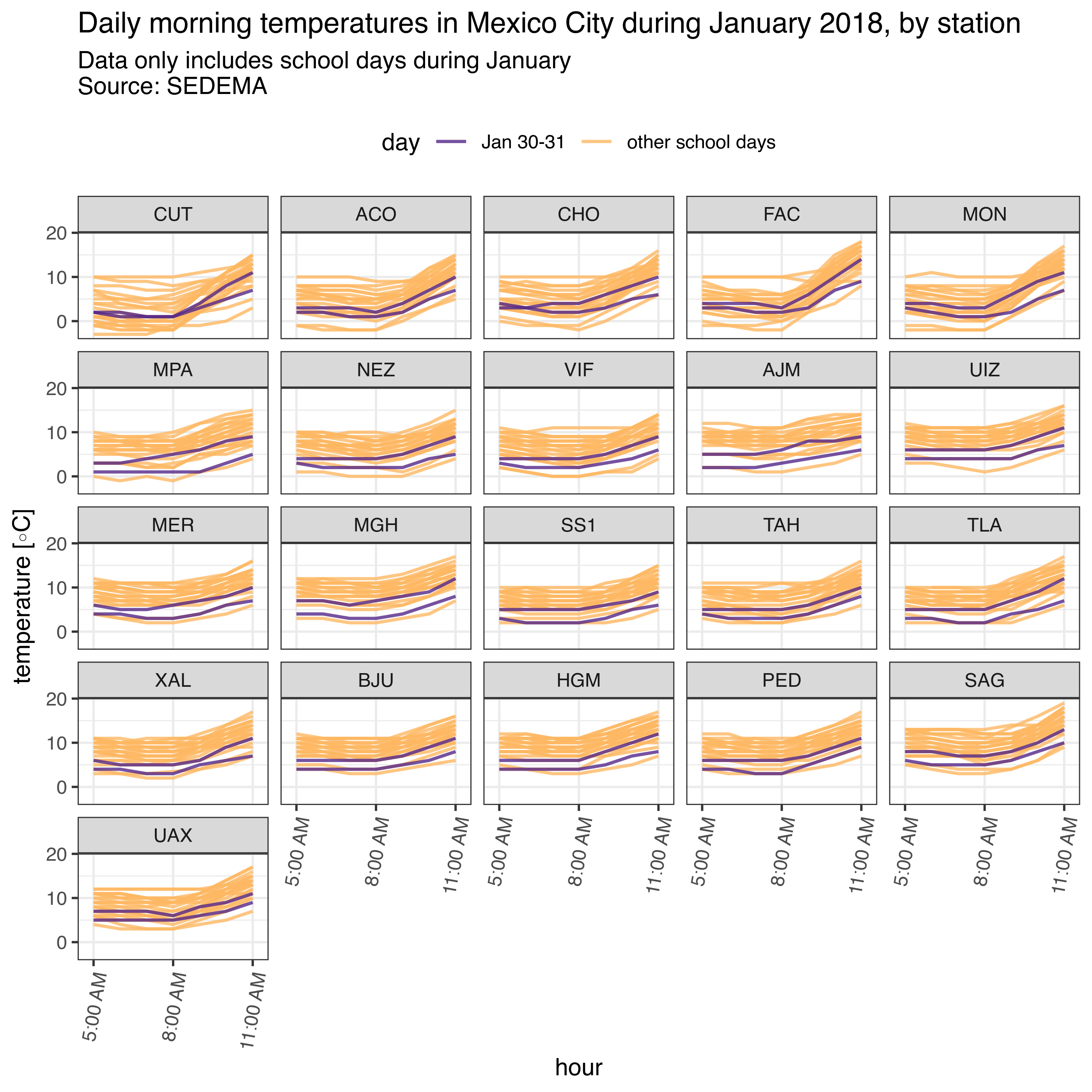
January Temperatures in 2018, by day

July 31, 2020

Data Aquisition

Data Cleaning

Plot