The Instituto Nacional de Ecología y Cambio Climático (INECC) created the SINAICA website to aggregate air quality data from monitoring stations across Mexico. This information is generated by local authorities and transmitted to SINAICA. This R package provides tools for downloading this data. In this example, we will use it to create a simple map of PM10 pollution in Guadalajara.
First, load the packages necessary for running the analysis
## Auto-install required R packages
packs <- c("dplyr", "ggplot2", "lubridate", "sp", "ggmap", "gstat", "zoo",
           "tidyr", "rsinaica")
load_pkg <- function(pkg) {
  suppressWarnings(require(pkg, character.only = TRUE))
}
success <- vapply(packs, load_pkg, logical(1))
missing <- packs[!success]
if (length(missing)) {
  install.packages(missing)
  vapply(missing, load_pkg, logical(1))
}
Core Functions
The basic function provided by the package:
-
sinaica_station_data(): Download data from a single station by specifying a parameter and a date range
This function can download the crude real-time data as it comes in, the older and not as complete validated data, or pollution data which is collected manually and sent to an external for lab analysis.
There are also two helper functions:
-
sinaica_station_dates(), which lists the dates for which a station has data available. -
sinaica_station_params(), which lists the air quality parameters measured at a station.
Downloading the data
We’ll use the sinaica_station_data function to download
pollution data for all the stations located in Guadalajara. We’ll use
the validated data to avoid having to filter values which are so far
outside the norm that they are obviously mistakes.
## Change this if you want a map of another city or parameter
parameter <- "PM10"
network <- "Guadalajara"
midpoint <- 76 # midpoint of regular air quality converted to IMECAs

## Download a single year of data for all Guadalajara stations
get_year <- function(start_date, end_date, net, parameter){
  bind_rows(
    lapply(
      stations_sinaica$station_id[stations_sinaica$network_name %in% net],
      sinaica_station_data,
      parameter,
      start_date,
      end_date,
      "Validated"
      )
  )
}
## Download 2023 data
df <- bind_rows(
  mapply(get_year,
         "2023-01-01",
         "2023-12-31",
         network,
         parameter,
         SIMPLIFY = FALSE)
  )
Here’s what the data we just downloaded looks like:
| id | date | hour | value | valid | unit | station_id | station_name |
|---|---|---|---|---|---|---|---|
| 101PM1023010100 | 2023-01-01 | 0 | NA | 1 | µg/m³ | 101 | Atemajac |
| 101PM1023010101 | 2023-01-01 | 1 | NA | 1 | µg/m³ | 101 | Atemajac |
| 101PM1023010102 | 2023-01-01 | 2 | NA | 1 | µg/m³ | 101 | Atemajac |
| 101PM1023010103 | 2023-01-01 | 3 | NA | 1 | µg/m³ | 101 | Atemajac |
| 101PM1023010104 | 2023-01-01 | 4 | NA | 1 | µg/m³ | 101 | Atemajac |
| 101PM1023010105 | 2023-01-01 | 5 | NA | 1 | µg/m³ | 101 | Atemajac |
Usually, for PM10 particles, a 24-hour average is taken as the current pollution value.
df <- df  %>%
  ungroup() %>%
  complete(station_id,
           hour = 0:23,
           date = as.character(seq(as.Date("2023-01-01"),
                                   as.Date("2023-12-31"),
                                   by = "day"))) %>%
  arrange(station_id, date, hour) %>%
  ungroup() %>%
  group_by(station_id) %>%
  mutate(roll24 = rollapply(value, 24, mean, na.rm = TRUE, partial = 12,
                            fill = NA, align = "right")) %>%
  select(-station_name) %>%
  left_join(stations_sinaica[,c("station_id", "station_name")],
            by = "station_id") %>%
  mutate(datetime = with_tz(as.POSIXct(paste0(date, " ", hour, ":00"),
                                  tz = "Etc/GMT+6"),
                       tz = "America/Mexico_City"))

ggplot(df, aes(datetime, roll24, group = station_name)) +
  geom_line(alpha = .8, size = .3) +
  ggtitle(expression(paste("24 hour average of ",
                           PM[10],
                           " data reported by Guadalajara stations"))) +
  xlab("date") +
  ylab(expression(paste("24 hr. average ", PM[10]," concentration in ppm"))) +
  facet_wrap(~ station_name) +
  theme_bw() +
  theme(axis.text.x=element_text(angle=70,hjust=1))
#> Warning: Using `size` aesthetic for lines was deprecated in ggplot2 3.4.0.
#> ℹ Please use `linewidth` instead.
#> This warning is displayed once per session.
#> Call `lifecycle::last_lifecycle_warnings()` to see where this warning was
#> generated.
#> Warning: Removed 21822 rows containing missing values or values outside the scale range
#> (`geom_line()`).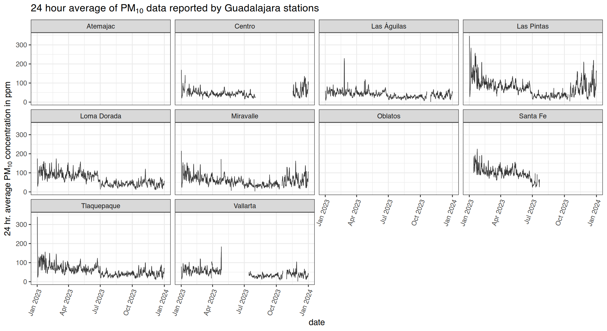
Grid of Guadalajara
We will use the longitude and latitude data of the measuring stations
in the stations_sinaica data.frame to create a grid
covering Guadalajara, and then extrapolate the pollution values to each
cell in the grid by inverse distance weighting from the values in the
locations of the measuring stations.
create_grid <- function(station_vec, pixels = 1000) {
df <- stations_sinaica[stations_sinaica$station_id %in% station_vec,]
geog <- df[,c("lat", "lon")]
coordinates(geog) <- ~lon+lat
proj4string(geog) <-
"+proj=longlat +datum=WGS84 +no_defs +ellps=WGS84 +towgs84=0,0,0"
## Add a margin surrounding the stations
geog@bbox <- bbox(geog) + c(-0.05, -0.05, 0.05, 0.05)
geog.grd <- makegrid(geog, n = pixels)
grd.pts <- SpatialPixels(SpatialPoints(geog.grd))
as(grd.pts, "SpatialGrid")
}
reporting_stations <- unique(df$station_id)
# 50x50 grid covering Guadalajara
grid <- create_grid(reporting_stations, 15000)
plot(grid,
main = paste0("Grid covering Guadalajara and Locations of",
"\nPollution Measuring Stations (red)"),
col = "#666666", lwd = .2)
# Plot the locations of the stations
geog <- stations_sinaica[stations_sinaica$station_id %in% reporting_stations,
c("lat", "lon", "station_code")]
coordinates(geog) <- ~lon+lat
points(geog, pch = 22, col = "lightgray", bg = "tomato1", cex = 1.2)
text(geog$lon, geog$lat, geog$station_code, pos = 1)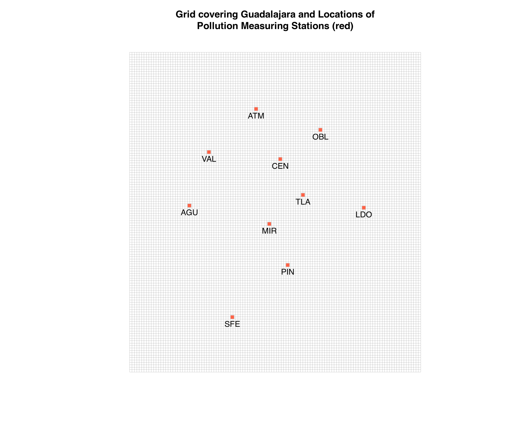 Now that the grid is ready we can use inverse distance to calculate the
pollution values in each grid cell.
Now that the grid is ready we can use inverse distance to calculate the
pollution values in each grid cell.
heatmap <- function(df, grid){
if(nrow(df) == 0){
return(data.frame(var1.pred = NA, var1.var = NA, lon = NA, lat = NA))
}
df <- left_join(df, stations_sinaica, by = "station_id")
df <- df[!is.na(df$value),]
df <- df[,c("lat", "lon", "value")]
coordinates(df) <- ~lon+lat
# For radiation pollution the exponent should be 2
# See http://www.sciencedirect.com/science/article/pii/S009830041200372X
df.idw <- idw(value ~ 1, df, grid, idp = 2, debug.level = 0)
idw <- as.data.frame(df.idw)
names(idw) <- c("var1.pred", "var1.var", "lon", "lat")
idw
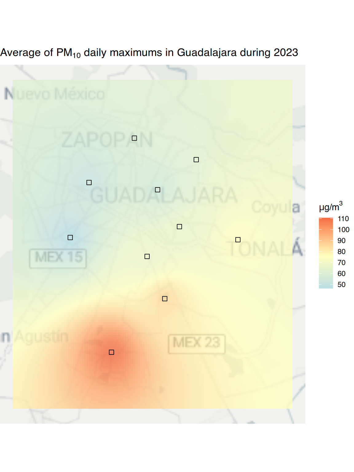
}We’ll show on the map the average of all the daily maximums of the twenty-four-hour rolling average of PM10 values.
df <- df %>%
  group_by(station_id, date) %>%
  summarise(maxroll24 = max(roll24, na.rm = TRUE)) %>%
  mutate(maxroll24 = if_else(!is.finite(maxroll24), NA_real_, maxroll24)) %>%
  group_by(station_id) %>%
  summarise(value = mean(maxroll24, na.rm = TRUE))
#> `summarise()` has regrouped the output.
#> ℹ Summaries were computed grouped by station_id and date.
#> ℹ Output is grouped by station_id.
#> ℹ Use `summarise(.groups = "drop_last")` to silence this message.
#> ℹ Use `summarise(.by = c(station_id, date))` for per-operation grouping
#>   (`?dplyr::dplyr_by`) instead.
idw_tiles <- heatmap(df, grid)
Plot
Now we will use the package ggmap to plot the locations
of the stations and the pollution grid on top of a map. Note that you’ll
need to set an environmental variable named STADIA_KEY with your Stadia
Maps api key (free
for non-commercial use)
# Signup for a free api key at: https://client.stadiamaps.com/signup
register_stadiamaps(Sys.getenv("STADIA_KEY"), write = FALSE)
qmplot(x1, x2, data = data.frame(grid), geom = "blank",
       maptype = "alidade_smooth", source = "stadia", zoom = 10)  +
  geom_tile(data = idw_tiles, aes(x = lon, y = lat, fill = var1.pred),
            alpha = .8) +
  ## set midpoint at 76 cause that's bad air quality according to
  ## http://www.aire.cdmx.gob.mx/default.php?opc=%27ZaBhnmI=&dc=%27aQ==
  scale_fill_gradient2(expression(paste(mu,"g/", m^3)),
                       low = "#abd9e9",
                       mid = "#ffffbf",
                       high = "#f46d43",
                       midpoint = midpoint) + # midpoint of regular air
                                              # quality converted from IMECAs
  geom_point(data = stations_sinaica[stations_sinaica$station_id %in%
                                       reporting_stations, ],
             aes(lon, lat), shape = 22, size = 2.6) +
  ggtitle(expression(paste("Average of ", PM[10],
                           " daily maximums in Guadalajara during 2023")))