Most Ozone-Polluted City in Mexico

We can use rsinaica to find out which city is the most ozone-polluted in all of Mexico.

First, we load the packages

## Auto-install required R packages
packs <- c("dplyr", "ggplot2", "gghighlight", "lubridate", "anomalize",
           "aire.zmvm", "tidyr", "zoo", "plotly", "rsinaica")
success <- suppressWarnings(sapply(packs, require, character.only = TRUE))
if (length(names(success)[!success])) {
  install.packages(names(success)[!success])
  sapply(names(success)[!success], require, character.only = TRUE)
}

Download

Then we download the data for the whole year of 2017 using the sinaica_param_data function. Since the maximum data range we can download is 1 month, we have to use a little mapply magic to download the entire year.

# Download all O3 pollution data in 2017
o3_2017 <- bind_rows(
  mapply(sinaica_param_data,
         "O3",
         seq(as.Date("2017-01-01"), as.Date("2017-12-01"), by = "month"),
         seq(as.Date("2017-02-01"), as.Date("2018-01-01"), by = "month") - 1,
         remove_extremes = FALSE,
         SIMPLIFY = FALSE)
)

This is what the data looks like:

knitr::kable(head(o3_2017))

id	station_id	station_name	station_code	network_name	network_code	network_id	date	hour	parameter	value_original	flag_original	valid_original	value_actual	valid_actual	date_validated	unit	value
101O317010100	101	Atemajac	ATM	Guadalajara	GDL	63	2017-01-01	0	O3	0.016239	128	1	0.016239	1	NA	ppm	0.0162390
101O317010101	101	Atemajac	ATM	Guadalajara	GDL	63	2017-01-01	1	O3	0.013322	128	1	0.013322	1	NA	ppm	0.0133220
101O317010102	101	Atemajac	ATM	Guadalajara	GDL	63	2017-01-01	2	O3	0.012865	128	1	0.012865	1	NA	ppm	0.0128650
101O317010103	101	Atemajac	ATM	Guadalajara	GDL	63	2017-01-01	3	O3	0.0070659	128	1	0.0070659	1	NA	ppm	0.0070659
101O317010104	101	Atemajac	ATM	Guadalajara	GDL	63	2017-01-01	4	O3	0.0021736	128	1	0.0021736	1	NA	ppm	0.0021736
101O317010105	101	Atemajac	ATM	Guadalajara	GDL	63	2017-01-01	5	O3	0.00066054	131	1	0.00066054	1	NA	ppm	0.0006605

Cleanup

Once we've downloaded the data we filter values below .3 ppm since they're probably calibration errors, and also filter some stations that never report correct ozone values. Given that ozone production depends on chemical reactions between oxides of nitrogen and volatile organic compounds in the presence of sunlight, it’s extremely unlikely to be present in large quantities at night or in the early morning, so we can filter high ozone values during those times.

# o3_2017[which(o3_2017$value_actual != o3_2017$value_original),]
# o3_2017[which(!is.na(o3_2017$date_validated)),]

# Only include stations that reported for more than 80% of days (292)
df_filtered <- o3_2017 %>%
  filter(!is.na(value)) %>%
  add_count(station_id, network_name) %>%
  ## these stations are mostly error values
  filter(!station_id %in% c(173, #"Facultad Psicología" SLP
                            72, #"Bomberos" Irapuato
                            31, #CBTIS ags 
                            303, #Instituto Educativo ags
                            39, #COCABH Mexicali
                            56 #Conalep torreon
                            )) %>%
  # filter values above .095 (bad (MALA) air quality)
  # that occurred during the night, since ozone is a photosensitive
  # pollutant
  filter(!(value > .0955 & hour %in% c(0:11, 21:23))) %>%
  filter(value < .3)

We'll be taking the average of the maximum daily value among all stations in each network for the entire year of 2017, and only include stations that reported data at least 80% of the days.

df_max <- df_filtered %>%
  group_by(date, network_name) %>%
  summarise(max = max(value, na.rm = TRUE)) %>%
  ungroup() %>%
  add_count(network_name) %>%
  filter(n > (365*.8))  %>%
  select(-n) %>%
  arrange(network_name)
#> `summarise()` regrouping output by 'date' (override with `.groups` argument)

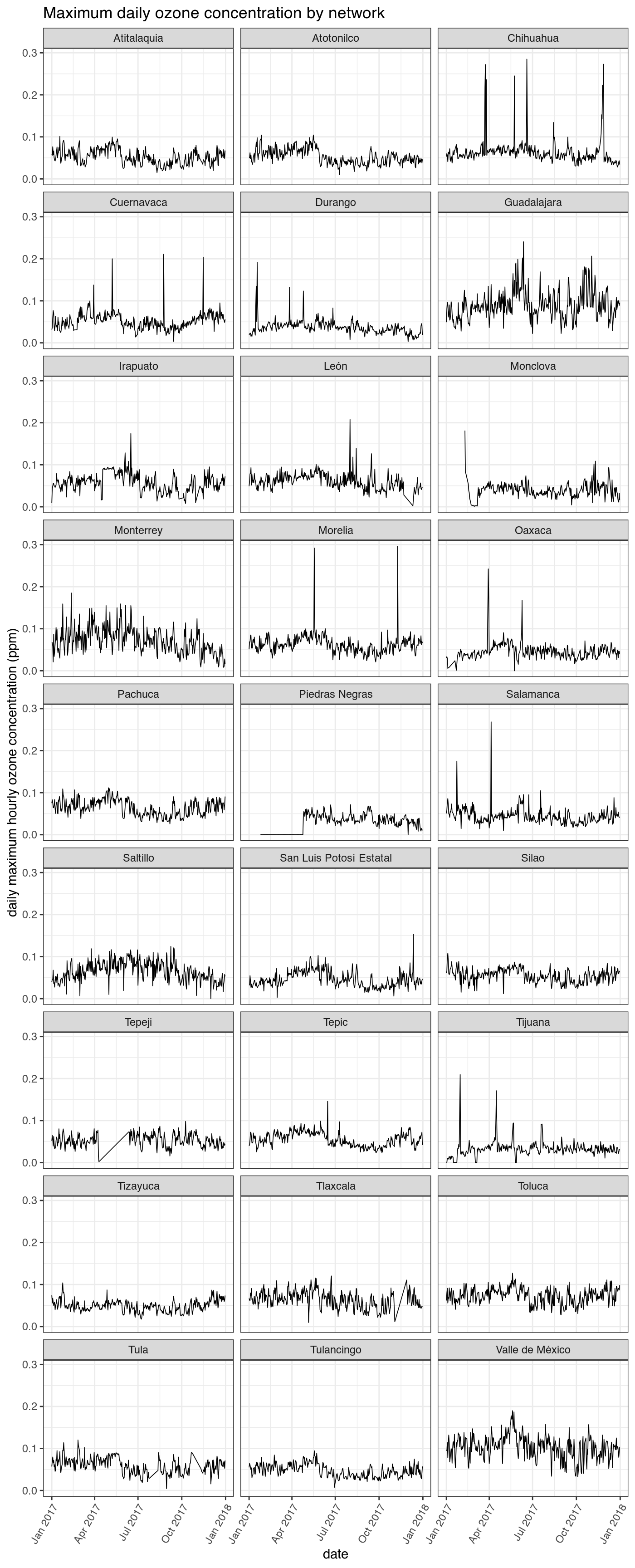
When plotting the daily maximums we can see that there are still some obvious errors in the data even after removing the stations that always report erroneous data and the extreme ozone values outside peak daylight hours.

ggplot(df_max, aes(as.Date(date), max)) +
  geom_line(size = .3, color = "black") +
  facet_wrap(~ network_name, ncol = 3) +
  ggtitle("Maximum daily ozone concentration by network") +
  xlab("date") +
  ylab("daily maximum hourly ozone concentration (ppm)") +
  theme_bw() +
  theme(axis.text.x=element_text(angle=60,hjust=1))

Anomalies

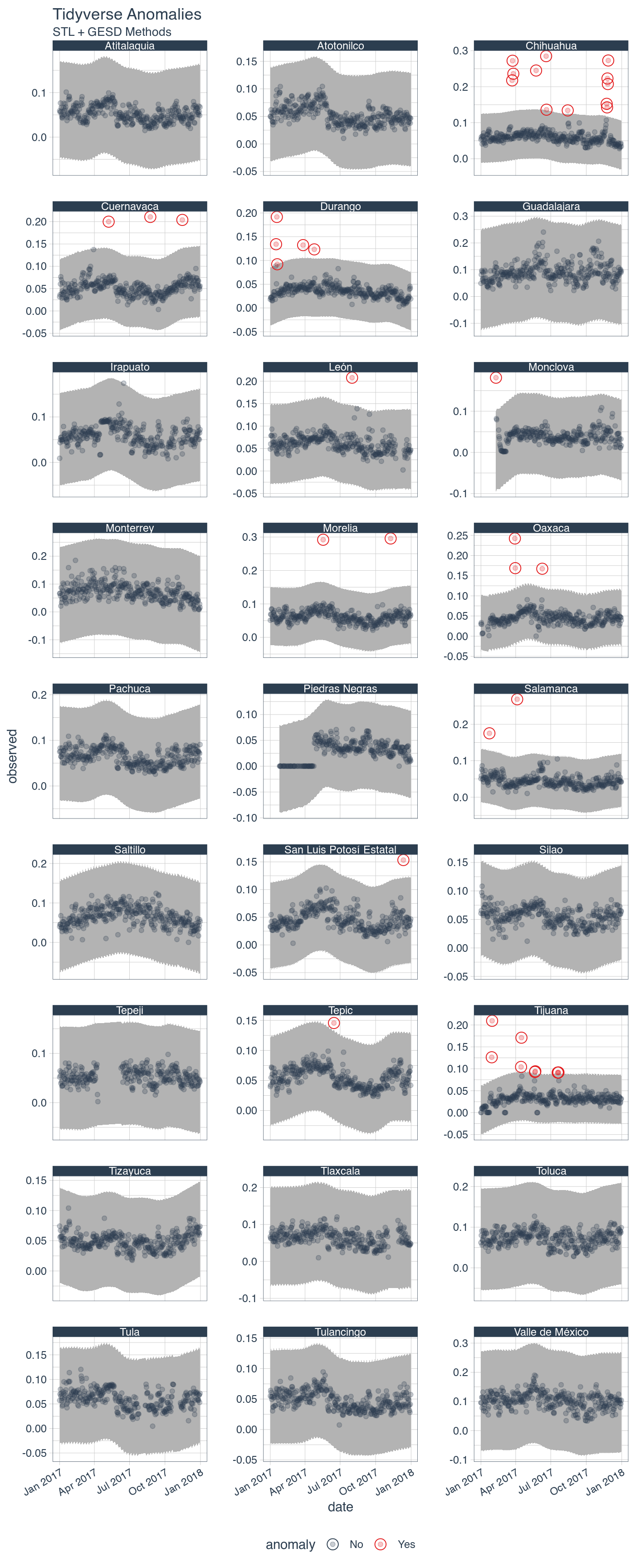
We can use the anomalize package to detect and remove the extreme values, while being careful not to remove the high ozone levels that happen in Mexico City, Guadalajara, and Monterrey.

df_max <- df_max %>%
  ungroup() %>%
  group_by(network_name) %>%
  mutate(date = as.Date(date)) %>%
  time_decompose(max) %>%
  anomalize(remainder, method = "iqr", alpha = .03) %>%
  time_recompose()
#> Registered S3 method overwritten by 'quantmod':
#>   method            from
#>   as.zoo.data.frame zoo

# Anomaly Visualization
df_max %>% plot_anomalies(time_recomposed = TRUE, ncol = 3, alpha_dots = 0.25) +
  labs(title = "Tidyverse Anomalies", subtitle = "STL + GESD Methods")

df_max <- filter(df_max, anomaly != "Yes")

Besides removing the outliers, after looking at the plots it was decided to remove the whole network of Piedras Negras since it only reported ozone concentrations close to zero during the first few months of 2017.

df_max <- filter(df_max, network_name != "Piedras Negras")

Most Ozone-Polluted City

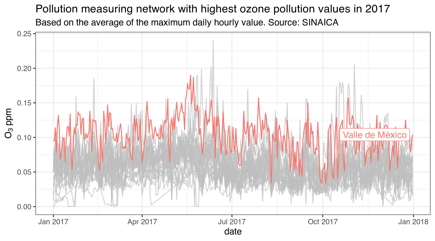
And here is the most ozone-polluted city in Mexico: the Valle de México metro area

ggplot(df_max, aes(as.Date(date), observed,
                   group = network_name, color = network_name)) +
  geom_line()  +
  theme_bw() +
  ggtitle("Pollution measuring network with highest ozone pollution values in 2017",
          subtitle = "Based on the average of the maximum daily hourly value. Source: SINAICA") +
  xlab("date") +
  ylab(expression(paste(O[3], " ppm"))) +
  gghighlight(mean(observed, na.rm = TRUE), max_highlight = 1L)
#> label_key: network_name

Top polluted cities

knitr::kable(
  df_max %>%
    group_by(network_name) %>%
    summarise(mean = mean(observed, na.rm = TRUE)) %>%
    arrange(-mean) %>%
    head(10)
  )
#> `summarise()` ungrouping output (override with `.groups` argument)

network_name	mean
Valle de México	0.1030799
Guadalajara	0.0900604
Toluca	0.0730411
Monterrey	0.0721818
Saltillo	0.0657089
Pachuca	0.0643098
Tlaxcala	0.0640684
Morelia	0.0615187
León	0.0607596
Tula	0.0600054

Perhaps not surprisingly, the most ozone-polluted cities in Mexico are also the among the most populous. It's kind of embarrassing that Puebla doesn't have a working air quality network since it is the fourth biggest metro area by population.

top3 <- filter(df_max, network_name %in% c("Valle de México",
                                           "Guadalajara",
                                           "Toluca"))[, 1:3]

top3 <- spread(top3, network_name, observed)
top3$date <- as.Date(as.Date(top3$date))
x <- list(
  title = "date"
)
y <- list(
  title = "daily maximum ozone concentration (ppm)"
)

plot_ly(as.data.frame(top3), x = ~date, y = ~`Valle de México`, name = "Valle de México" ,
        type = 'scatter', mode = 'lines', line = list(color = '#e41a1c'), width = .5) %>%
  add_trace(y = ~Guadalajara, name = 'Guadalajara', mode = 'lines', line = list(color = '#377eb8'), width = .5) %>%
  add_trace(y = ~Toluca, name = 'Toluca', mode = 'lines', line = list(color = '#4daf4a'), width = .5) %>%
  layout(title = "Top 3 most ozone-polluted cities in Mexico", xaxis = x, yaxis = y)

Days with bad air quality

Number of days with bad air quality (Índice IMECA MALO)

df_max %>%
  group_by(network_name) %>%
  filter(observed > 95.5/1000 ) %>%
  summarise(count = n()) %>%
  arrange(-count) %>%
  head() %>%
  knitr::kable()
#> `summarise()` ungrouping output (override with `.groups` argument)

network_name	count
Valle de México	233
Guadalajara	130
Monterrey	78
Toluca	41
Saltillo	38
Tlaxcala	18

Number of days with very bad air quality (Índice IMECA MUY MALO).

df_max %>%
  group_by(network_name) %>%
  filter(observed > 155/1000) %>%
  summarise(count = n()) %>%
  arrange(-count) %>%
  head() %>%
  knitr::kable()
#> `summarise()` ungrouping output (override with `.groups` argument)

network_name	count
Guadalajara	21
Valle de México	10
Monterrey	4
Irapuato	1

Here we see that Guadalajara actually had more very bad days. If this had happened in Mexico City, a phase I smog alert would have been issued and 40% of cars would have been banned from taking to the roads, but Guadalajarans are to smart to implement something like this, since it doesn't seem to work.

Most Ozone-Polluted City in Mexico - 2017