With rsinaica we can plot the long term trends in pollution for different cities. First, we load the packages
## Auto-install required R packages
packs <- c("dplyr", "ggplot2", "lubridate", "scales", "rsinaica")
success <- suppressWarnings(sapply(packs, require, character.only = TRUE))
if (length(names(success)[!success])) {
  install.packages(names(success)[!success])
  sapply(names(success)[!success], require, character.only = TRUE)
}
We create a function for downloading single pollutant data for all the stations that form a network
get_network_data <- function(network_name, pollutant, remove_extremes = TRUE) {
  ## Download data for all Aguascalientes stations for a single month
  get_month <- function(start_date, end_date, net){
    bind_rows(
      lapply(stations_sinaica$station_id[stations_sinaica$network_name %in% net],
             sinaica_station_data, pollutant, start_date, end_date, "Crude",
             remove_extremes = remove_extremes)
    )
  }
  ## Download data for 2017, by month
  df <- bind_rows(
    mapply(get_month,
           seq(as.Date("1997-01-01"), as.Date("2017-12-01"), by = "month"),
           seq(as.Date("1997-02-01"), as.Date("2018-01-01"), by = "month") - 1,
           network_name,
           SIMPLIFY = FALSE)
  )

  df$datetime <-  with_tz(as.POSIXct(paste0(df$date, " ", df$hour, ":00"),
                                     tz = "Etc/GMT+6"),
                          tz = "America/Mexico_City")
  df
}
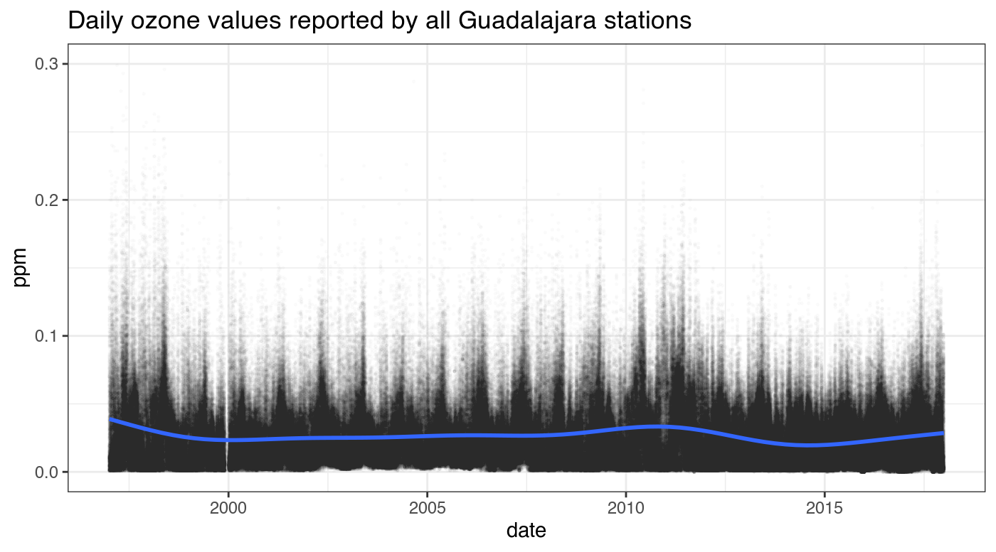
Now we are ready to plot different cities. When requesting ozone values with the sinaica_station_data function, there is an option to automatically clean the data and set values above .2 ppm to NA, since Guadalajara tends to have quite high ozone levels it is probably a good idea to disable this functionality.
get_network_data("Guadalajara", "O3", remove_extremes = FALSE) %>%
  ## remove ozone values above .3 cause Guadalajara air is extremely dirty
  filter(value < .3 & value >= 0) %>%
  ggplot(aes(as.Date(date), value)) +
  geom_point(alpha = .01, size = .3) +
  geom_smooth(method = 'gam', formula = y ~ s(x)) +
  ggtitle("Daily ozone values reported by all Guadalajara stations") +
  xlab("date") +
  ylab("ppm") +
  coord_cartesian(ylim = c(0, 0.3)) +
  theme_bw()
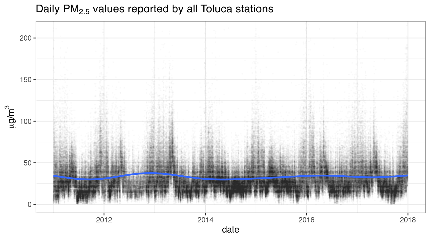
get_network_data("Toluca", "PM2.5", remove_extremes = FALSE) %>%
  filter(value <= 750) %>%
  ggplot(aes(as.Date(date), value)) +
  geom_point(alpha = .01, size = .3) +
  geom_smooth(method = 'gam', formula = y ~ s(x)) +
  ggtitle(expression(paste("Daily ", PM[2.5],
                           " values reported by all Toluca stations"))) +
  xlab("date") +
  ylab(expression(paste(mu,"g/", m^3))) +
  coord_cartesian(ylim = c(0, 210)) +
  theme_bw()
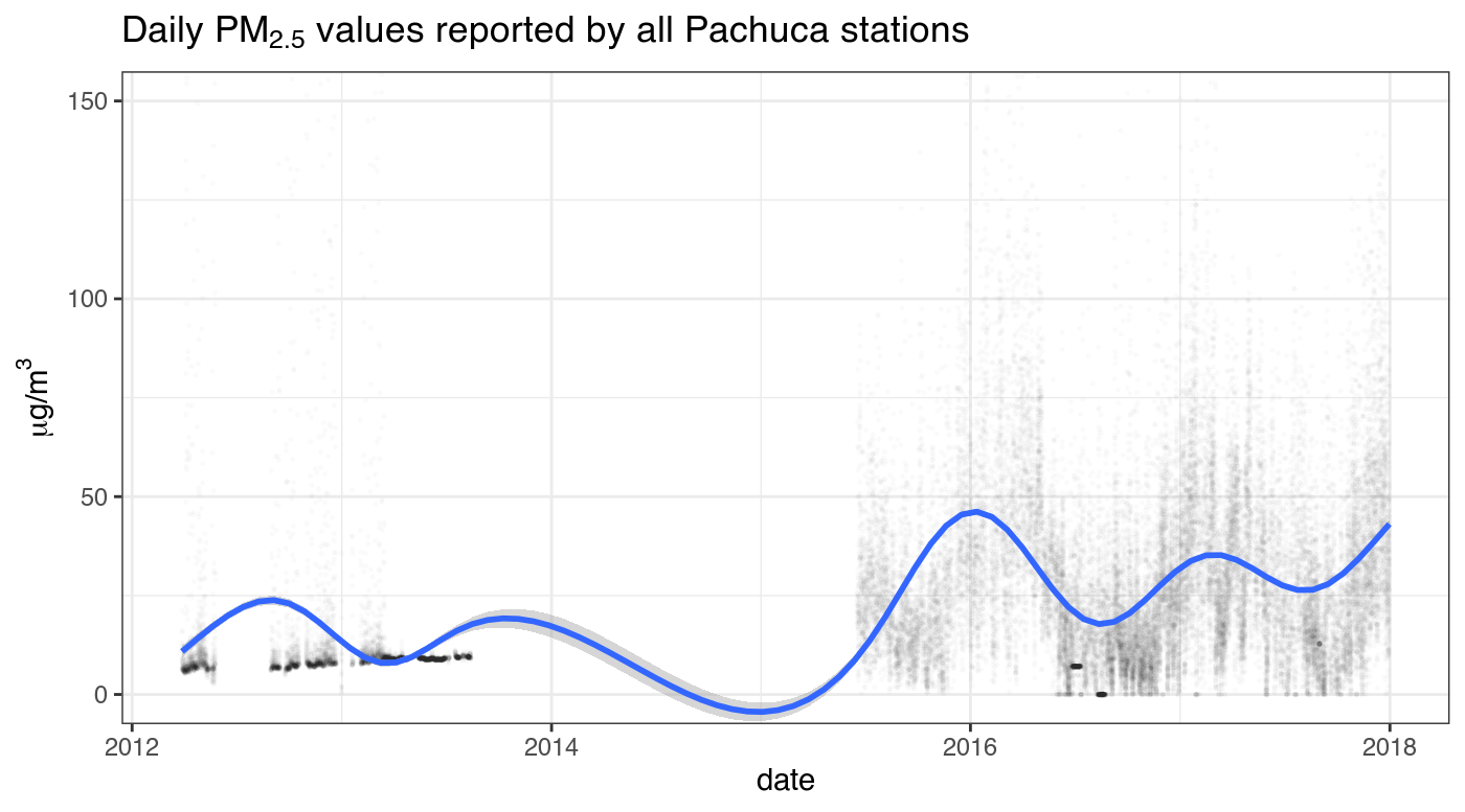
get_network_data("Pachuca", "PM2.5", remove_extremes = FALSE) %>%
  filter(value <= 600) %>%
  ggplot(aes(as.Date(date), value)) +
  geom_point(alpha = .01, size = .3) +
  geom_smooth(method = 'gam', formula = y ~ s(x)) +
  ggtitle(expression(paste("Daily ", PM[2.5],
                           " values reported by all Pachuca stations"))) +
  xlab("date") +
  ylab(expression(paste(mu,"g/", m^3))) +
  coord_cartesian(ylim = c(0, 150)) +
  theme_bw()
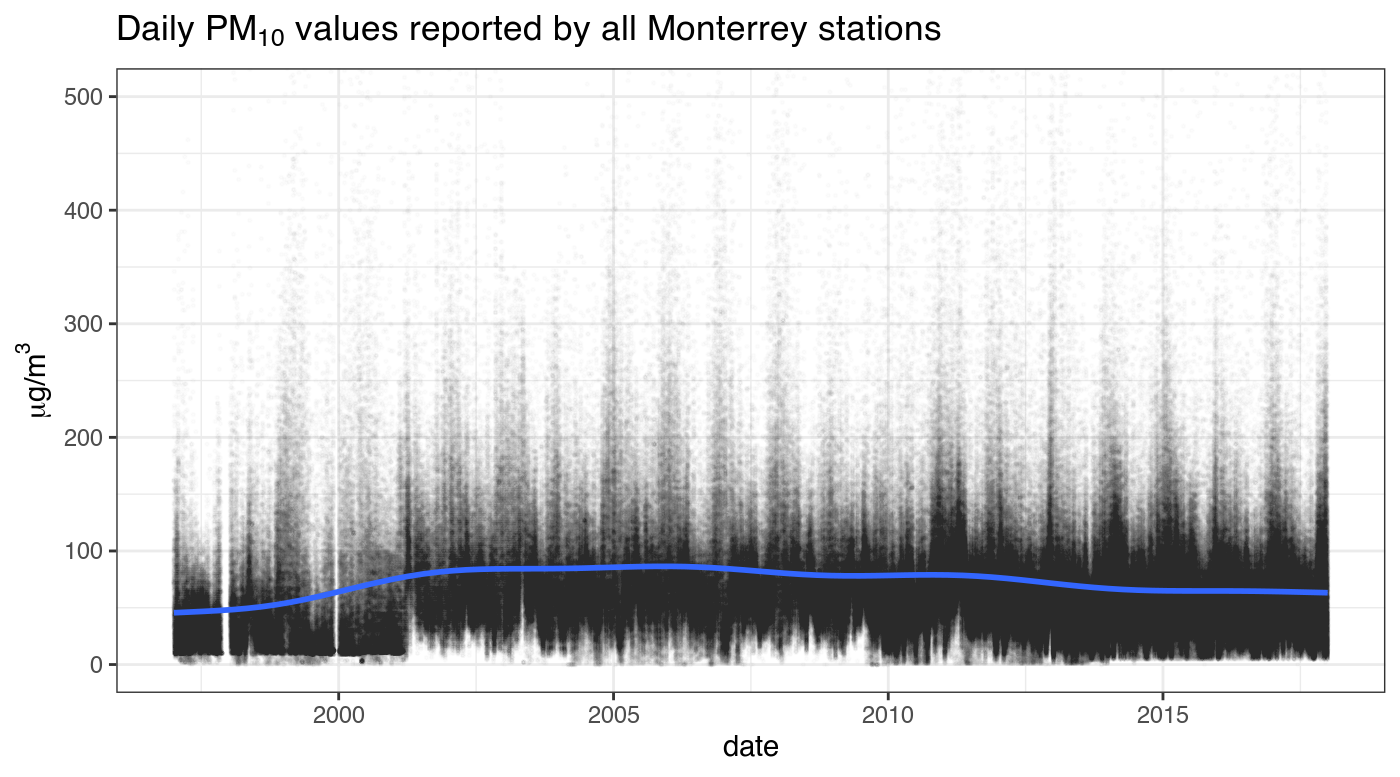
get_network_data("Monterrey", "PM10", remove_extremes = FALSE) %>%
  filter(value <= 1000) %>%
  ggplot(aes(as.Date(date), value)) +
  geom_point(alpha = .01, size = .3) +
  geom_smooth(method = 'gam', formula = y ~ s(x)) +
  ggtitle(expression(paste("Daily ", PM[10],
                           " values reported by all Monterrey stations"))) +
  xlab("date") +
  ylab(expression(paste(mu,"g/", m^3))) +
  coord_cartesian(ylim=c(0, 500)) +
  theme_bw()