Comparing rsinaica to aire.zmvm
Diego Valle-Jones
2020-08-08
Source:vignettes/articles/airezmvm_vs_rsinaica.Rmd
airezmvm_vs_rsinaica.RmdWe can compare the data available from rsinaica to that of aire.zmvm by downloading data from the same station. In this example we'll download data from the Xalostoc station in Mexico City. First, we load the necessary packages:
## Auto-install required R packages
packs <- c("dplyr", "ggplot2", "lubridate", "aire.zmvm", "rsinaica")
success <- suppressWarnings(sapply(packs, require, character.only = TRUE))
if (length(names(success)[!success])) {
  install.packages(names(success)[!success])
  sapply(names(success)[!success], require, character.only = TRUE)
}
The hourly data from the aire.zmvm package in most cases corresponds to the GMT+6 time zone (with no Daylight Saving Time), while according to the stations_sinaica data.frame the data for the Xalostoc station comes in the local Mexico City time that includes Daylight Saving Time during the summer. Be warned that each station submits its data to SINAICA according to their chosen time zone, and sometimes the reported time zone may be incorrect.
## 271 is the station_id of Xalostoc
stations_sinaica$timezone[stations_sinaica$station_id == 271]
#> [1] "Tiempo del centro, UTC-6 (UTC-5 en verano)"
Then we download the data and make sure that both the values from aire.zmvm and rsinaica are in ppb (parts per billion), since rsinaica returns values in ppm (parts per million) we multiply by 1,000.
df_aire <- get_station_month_data("HORARIOS", "O3", 2017, 5) %>%
  filter(station_code == "XAL") %>%
  mutate(value_aire.zmvm = value)
## data from get_station_month_data is in GMT+6
df_aire$datetime <-  as.POSIXct(
  strptime(paste0(df_aire$date, " ", df_aire$hour),
           "%Y-%m-%d %H", tz = "Etc/GMT+6")
)
df_aire <- df_aire[, c("datetime", "value_aire.zmvm")]


## values from sinaica are in ppb and those from aire.cdmx in ppm
## Xalostoc station has an rsinaica station_id of 271
df_sinaica <- sinaica_station_data(271, "O3", "2017-05-01", "2017-05-31") %>%
  mutate(value = value * 1000) %>%
  mutate(value_sinaica = value) %>%
  mutate(date = as.Date(date))
## data from rsinaica is in the local Mexico City time zone
df_sinaica$datetime <-  as.POSIXct(
  strptime(paste0(df_sinaica$date, " ", df_sinaica$hour),
           "%Y-%m-%d %H", tz = "America/Mexico_City")
)
df_sinaica <- df_sinaica[, c("datetime", "value_sinaica")]

df <- full_join(df_aire, df_sinaica, by = c("datetime" = "datetime"))
This is what the merged data looks like:
| datetime | value_aire.zmvm | value_sinaica | |
|---|---|---|---|
| 5 | 2017-05-01 05:00:00 | 2 | 2 |
| 6 | 2017-05-01 06:00:00 | 2 | 2 |
| 7 | 2017-05-01 07:00:00 | 3 | 3 |
| 8 | 2017-05-01 08:00:00 | 5 | 5 |
| 9 | 2017-05-01 09:00:00 | 17 | 17 |
| 10 | 2017-05-01 10:00:00 | 55 | 55 |
and the mean squared error:
mean((df$value_aire.zmvm - df$value_sinaica)^2, na.rm = TRUE)
#> [1] 22.01807
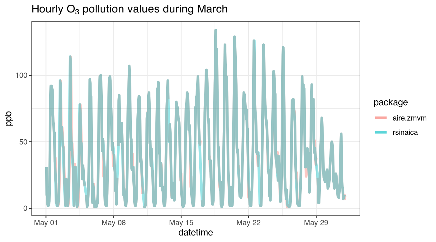
We can visually compare them with a plot. The values are extremely similar, but the aire.zmvm data is a little bit more accurate since it comes directly from the source.
ggplot(df_aire, aes(datetime, value_aire.zmvm, color = "aire.zmvm")) +
  geom_line(size = 1.5, alpha = .4) +
  geom_line(data = df_sinaica, aes(datetime, value_sinaica, color = "rsinaica"),
            alpha = .4, size = 1.5) +
  xlab("datetime") +
  ylab("ppb") +
  scale_color_discrete("package") +
  ggtitle(expression(paste("Hourly ", O[3], " pollution values during March"))) +
  theme_bw()